2 Exploring Basketball Shots Data
Note that all the R code used in this book is accessible on GitHub.
2.1 Tracking Basketball Shots
Basketball shot coordinates1 can be tracked manually using pen and paper. The \((x, ~y)\) coordinates of each dot could be estimated once a reference frame for the basketball court has been chosen. Let's consider a FIBA basketball court (exact dimensions can be found here). We can focus on the half-court for now and set the origin of our two-dimensional coordinate system at the bottom left corner of the image below.
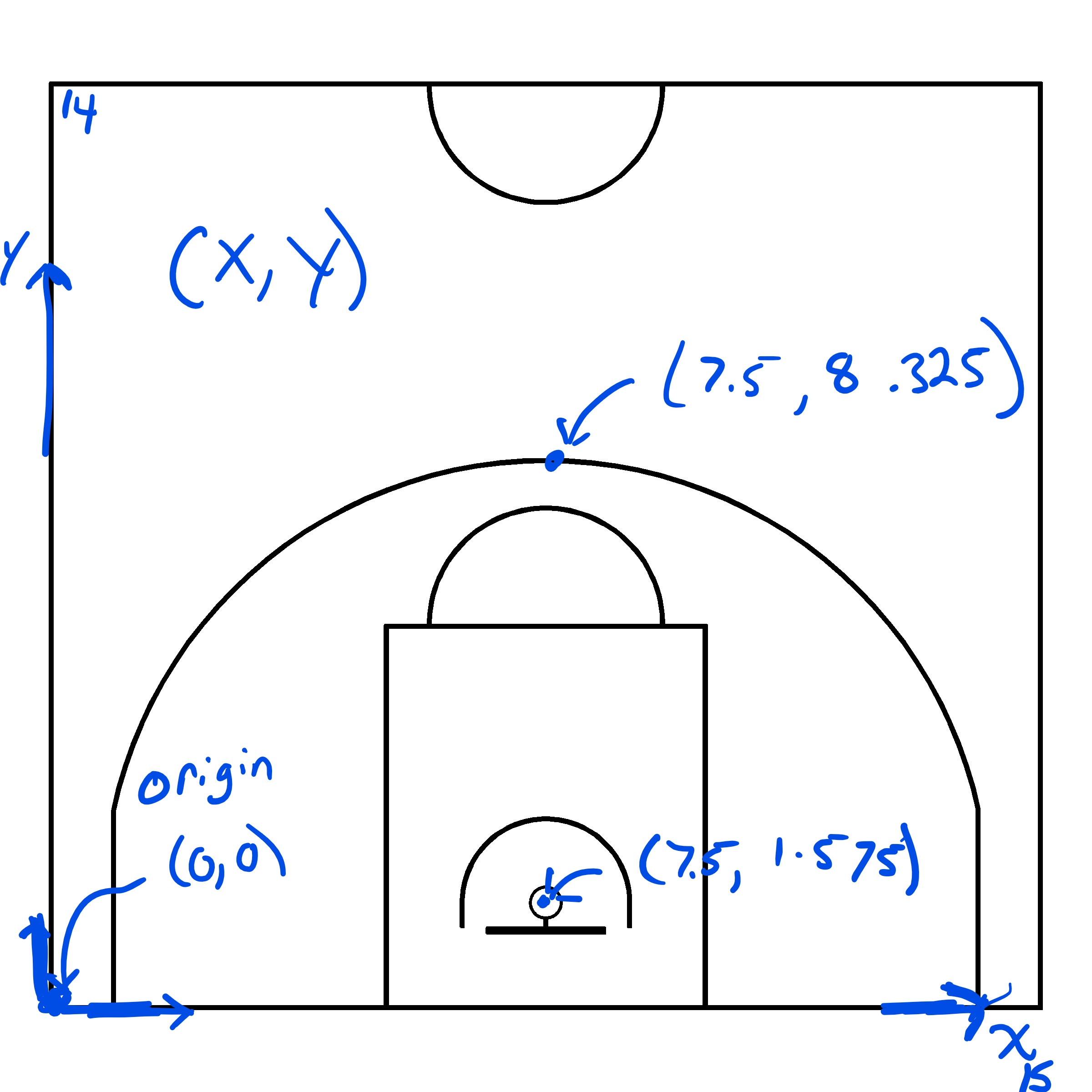
Once we've picked a coordinate system, then we could visually estimate the \((x, ~y)\) coordinates of each shot that was tracked on paper. Of course, this is not ideal. I built this Desmos file in the early days to manually estimate the shot coordinates.
This is where the Easy Stats iOS application comes in. You can watch this video tutorial to see how one can easily track and export more precise shot coordinates. In short, we can use the app to keep track of the shooter, the outcome of the shot (made or missed), and the location of the shot. This play-by-play data can be exported as a csv file via email.
2.2 Getting To Know Our Data
A basic shot data set was put together for this analysis. Let's see what we're working with.
# Load the tidyverse library to be able to use %>% and dplyr to wrangle
library(tidyverse)

# Load the artificial shot data
shots <- readRDS(file = "data/shots.rds")

# Display the general structure of the data and the first few observations
glimpse(shots)
## Rows: 1,163
## Columns: 4
## $ player <fct> Player 7, Player 3, Player 7, Player 3, Player 13, P~
## $ shot_made_numeric <dbl> 1, 0, 1, 0, 0, 0, 1, 1, 1, 0, 1, 0, 0, 1, 0, 0, 0, 0~
## $ loc_x <dbl> 4.386864, 5.779800, 3.003072, 3.377976, 3.161568, 3.~
## $ loc_y <dbl> 7.955280, 8.510016, 7.083552, 7.202424, 7.202424, 7.~We see from the output above that we have shots for 18 players in our data set. The \(x\) component of the location seems to stay between 0 and 15. This makes sense since the data set was created using a FIBA sized basketball court which has a width of 15 meters and a height of 28 meters. It therefore makes sense that highest recorded shot had a \(y\) component of 9.8 meters given that the three-point is 8.325 meters from the baseline.
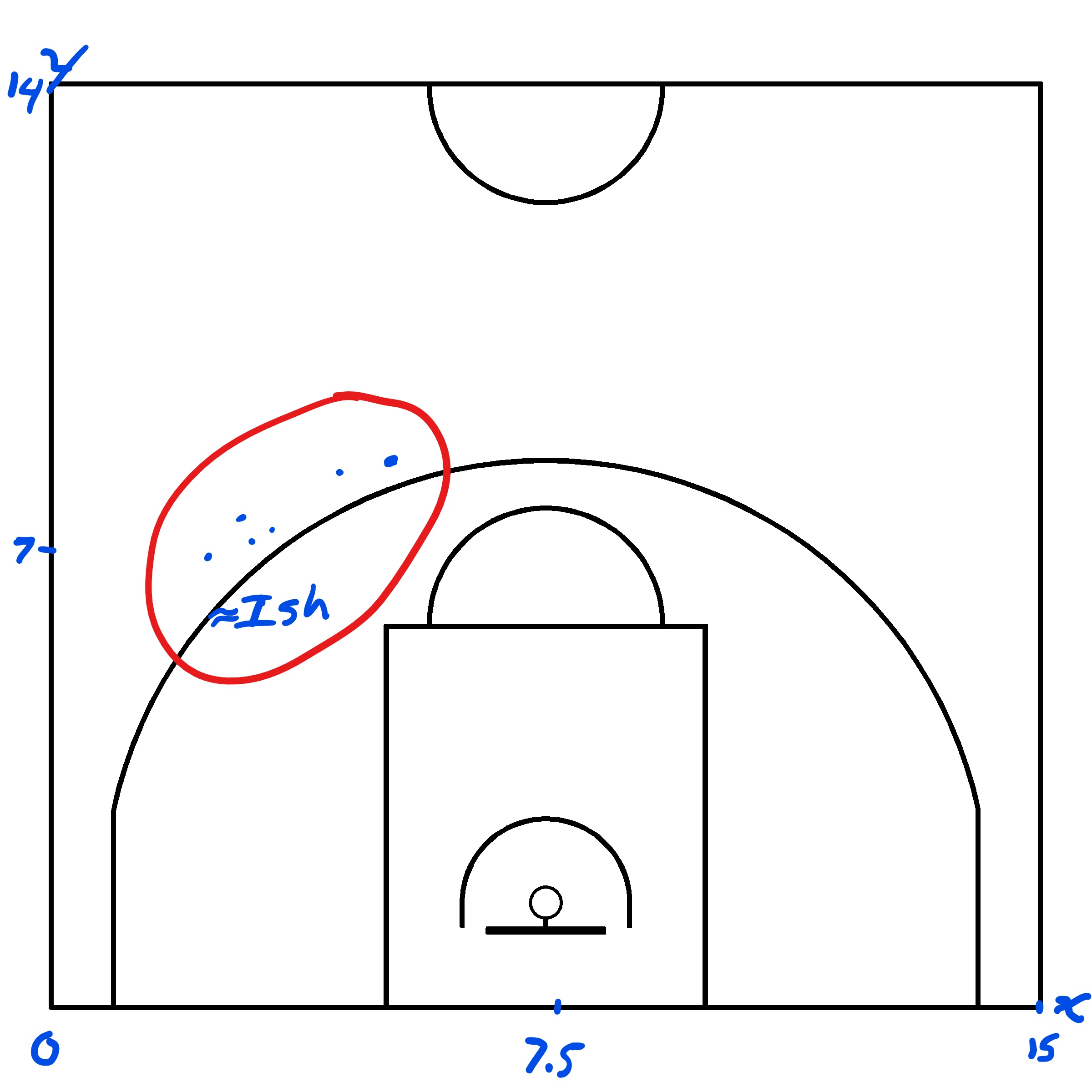
Lastly, we can see that Player 7 made their first shot at location \((4.39, 7.96)\). We can try to place this first shot on a basketball court. We know that \(4.39 < 7.5\) which implies that the shot was taken on the right side of the court from the players perspective looking at the rim. The picture below shows the estimated location of the first six shots.
2.3 Augmenting Our Data
We need to create a FIBA basketball court in R to plot these points exactly. But first, let's add a few columns to hour data. We can convert the player variable to a factor variable and reorder it's levels. We can create a factor variable for the binary outcome of whether the shot was made or not and properly label its levels.
# Add a few variables and clean others
shots <- shots %>%
  # Convert shots to a tibble format
  tibble() %>%
  # Add Columns
  mutate(
    # convert players to a factor
    player =  factor(
      player,
      # Re-level P1, P2, ..., P18
      levels = paste("Player", 1:length(unique(shots$player)))
      ),
    # Create  a factor binary variable for whether the shot was made or not
    shot_made_factor = recode_factor(factor(shot_made_numeric),
      "0" = "Miss",
      "1" = "Make"
      )
  )

# Display the first few rows
head(shots)
## # A tibble: 6 x 5
## player shot_made_numeric loc_x loc_y shot_made_factor
## <fct> <dbl> <dbl> <dbl> <fct>
## 1 Player 7 1 4.39 7.96 Make
## 2 Player 3 0 5.78 8.51 Miss
## 3 Player 7 1 3.00 7.08 Make
## 4 Player 3 0 3.38 7.20 Miss
## 5 Player 13 0 3.16 7.20 Miss
## 6 Player 7 0 3.33 7.14 Miss2.3.1 Shot Distance
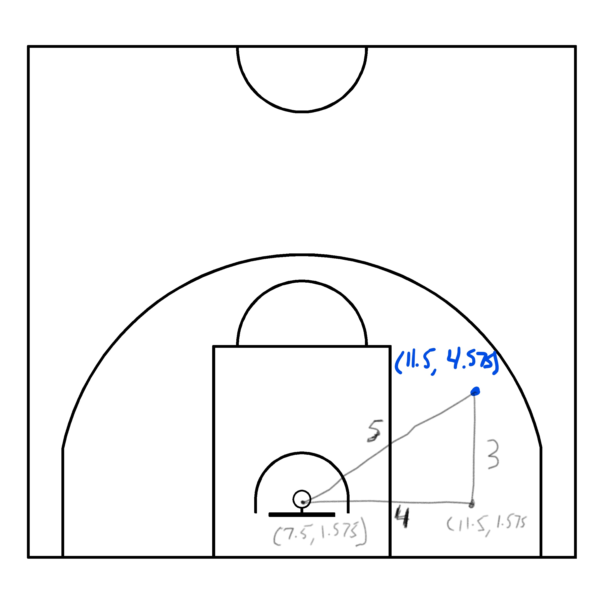
We can calculate the 2D distance between each shot \((x, ~y)\) coordinates and the center of the hoop located at \((7.5, ~1.575)\). Note that our coordinate reference system (crs) is measured in meters. To do so, we can use the distance formula.
\[ d = \sqrt{(x - 7.5)^2 + (y - 1.575)^2} \] Note that this formula for distance works since it is essentially the Pythagorean Theorem. Consider the simplistic example of a shot located at \((11.5, ~4.575)\). You can use the formula to calculate the distance or you can see from the image below that the distance should be 5 meters by the Pythagorean Theorem.
We can convert a distance from meters to feet with the following equivalence.
\[ d_{\mbox{feet}} = d_{\mbox{meters}} \times \left( 3.28084 ~ \frac{\mbox{ft}}{\mbox{m}} \right) \]
# Define FIBA court width and y-coordinate of hoop center in meters
width <- 15
hoop_center_y <- 1.575

# Calculate the shot distances
shots <- shots %>%
  # Add Columns
  mutate(
    dist_meters = sqrt((loc_x-width/2)^2 + (loc_y-hoop_center_y)^2),
    dist_feet = dist_meters * 3.28084
  )

# Display the first few rows
head(shots)
## # A tibble: 6 x 7
## player shot_made_numeric loc_x loc_y shot_made_factor dist_meters dist_feet
## <fct> <dbl> <dbl> <dbl> <fct> <dbl> <dbl>
## 1 Player 7 1 4.39 7.96 Make 7.10 23.3
## 2 Player 3 0 5.78 8.51 Miss 7.15 23.4
## 3 Player 7 1 3.00 7.08 Make 7.11 23.3
## 4 Player 3 0 3.38 7.20 Miss 6.98 22.9
## 5 Player 13 0 3.16 7.20 Miss 7.11 23.3
## 6 Player 7 0 3.33 7.14 Miss 6.96 22.82.3.2 Shot Angle
We can also calculate the angle \(\theta\) between the line going through the shot location and the center of the hoop and the vertical center line located at \(x = 7.5\). Looking at the diagram below is almost certainly a better way to grasp how we defined the shot angle.
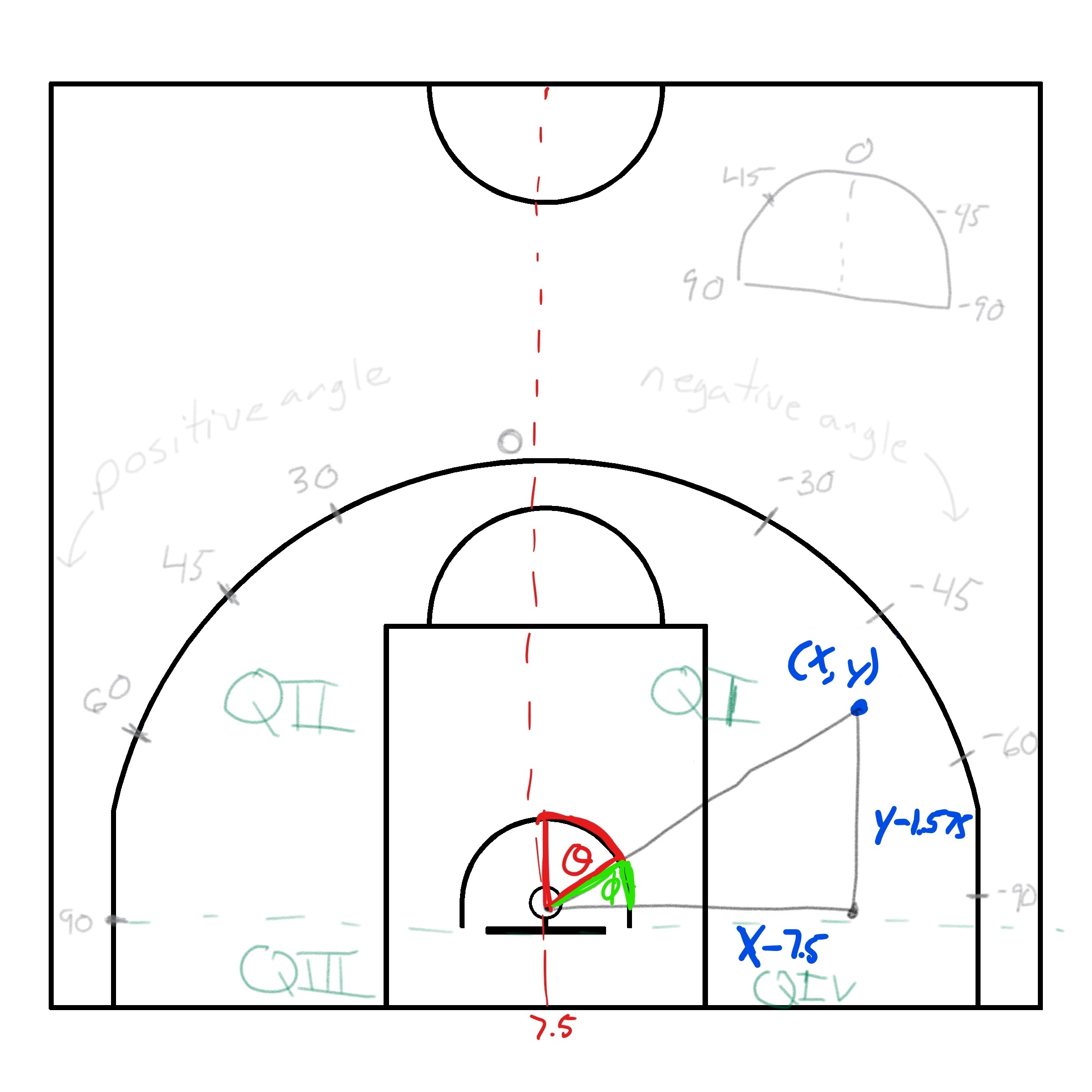
We see that the shot angle is \(\theta\) (red). To calculate it, we could calculate \(\phi\) (green) and subtract it from \(90^{\circ}\) or \(\frac{\pi}{2}\) radians. We can use SOH CAH TOA to calculate \(\phi\). Since we have the opposite and adjacent sides to the angle \(\phi\), we can use the tangent ratio (\(\tan(\phi) = \frac{O}{A}\)). Thus, we get that \(\phi = \arctan(\frac{y - 1.575}{x - 7.5})\). Then, we have \(\theta = \phi - \frac{\pi}{2}\) for the shot in the picture above. Note that the shot angle is negative since we defined shots on the left-hand side of the court (from the player's perspective) to have negative angle values. Note that how exactly we calculate this angle will depend on which quadrant is the shot is released from but the same logic applies. By default, most calculators will return angles in radians. We can easily convert the angles to degrees by using the following equivalence.
\[ \theta_{\mbox{degrees}} = \theta_{\mbox{radians}} \times \left( \frac{180 ~ \mbox{degrees}}{\pi ~ \mbox{radians}} \right) \]
# Calculate the shot angles
shots <- shots %>%
  # Add Columns
  mutate(
    theta_rad = case_when(
      # Quadrant 1: Shots from left side higher than the rim
      loc_x > width/2 & loc_y > hoop_center_y ~ atan((loc_x-width/2)/(loc_y-hoop_center_y)),
      # Quadrant 2: Shots from right side higher than the rim
      loc_x < width/2 & loc_y > hoop_center_y ~ atan((width/2-loc_x)/(loc_y-hoop_center_y)),
      # Quadrant 3: Shots from right side lower than the rim
      loc_x < width/2 & loc_y < hoop_center_y ~ atan((hoop_center_y-loc_y)/(width/2-loc_x))+(pi/2),
      # Quadrant 4: Shots from left side lower than the rim
      loc_x > width/2 & loc_y < hoop_center_y ~ atan((hoop_center_y-loc_y)/(loc_x-width/2))+(pi/2),
      # Special Cases
      loc_x == width/2  & loc_y >= hoop_center_y ~ 0, # Directly centered front
      loc_x == width/2  & loc_y < hoop_center_y ~ pi, # Directly centered back
      loc_y == hoop_center_y ~ pi/2, # Directly parallel to hoop center
    ),
    # Make the angle negative if the shot is on the left-side
    theta_rad = ifelse(loc_x > width/2, -theta_rad, theta_rad),
    # Convert the angle from radians to degrees
    theta_deg = theta_rad * (180/pi)
  )

# Display the first few rows
head(shots) %>%
  # Only display a few columns
  select(player, dist_meters, dist_feet, theta_rad, theta_deg)
## # A tibble: 6 x 5
## player dist_meters dist_feet theta_rad theta_deg
## <fct> <dbl> <dbl> <dbl> <dbl>
## 1 Player 7 7.10 23.3 0.454 26.0
## 2 Player 3 7.15 23.4 0.243 13.9
## 3 Player 7 7.11 23.3 0.685 39.2
## 4 Player 3 6.98 22.9 0.632 36.2
## 5 Player 13 7.11 23.3 0.657 37.6
## 6 Player 7 6.96 22.8 0.643 36.8
# Save the augmented data
saveRDS(shots, file = "data/shots_augmented.rds")
Note that all the R code used in this book is accessible on GitHub.