I love poker. It strikes a balance between skill and luck. A complete beginner can theoretically beat the world’s best player. In the long run, however, the skilled player will always come out on top. My statistics and mathematics background is the ideal skill set to master the game of poker. That said, it is the psychological and game theoretical aspect of the game that fascinates me. In this article, we’ll explore the bankroll management strategies that I use to avoid going broke.
The typical format for one of our poker nights is to get approximately 6 players who buy in with 20$. The total pot is hence 120$. Usually, we would distribute the prizes as follows:
- First place: 90$
- Second place: 30$
- How big of a bankroll do we need to be 99% sure of not going broke?
Note that the last two players can agree to split the pot how they see fit.
Based on historical data, I estimated that my chances of finishing in each position look something like this:
| Position | Probability | Prize | Profit |
| First | 20% | 90$ | 70$ |
| Second | 20% | 30$ | 10$ |
| Third | 20% | 0$ | -20$ |
| Fourth | 15% | 0$ | -20$ |
| Fifth | 15% | 0$ | -20$ |
| Sixth | 10% | 0$ | -20$ |
Note that this results in a 40% chance of making a profit and a 60% of losing the initial buy-in of 20$. We can calculate the chances that I lose K times in a row.
| Consecutive Losses | Probability |
| 1 |  |
| 2 |  |
| 3 |  |
| 4 |  |
| 5 |  |
| 6 |  |
Someone with my skill level and a 100$ bankroll (budget) for poker nights has a high risk (8%) of going broke playing 20$ buy-in tables. Another way to analyze the results is through the lens of expected value.
Expected Value
My expected value (EV) for this given format represents the average amount of money I can expect to win per poker night in the long run. The expected value formula is  . In words, we need to multiply the probabilities by the profits and add them.
![\[0.2\cdot70+0.2\cdot10+0.6\cdot-20 = 4\$\]](https://duddhawork.com/wp-content/ql-cache/quicklatex.com-058af3d58bad583aa9ee0e0ed7d7ae40_l3.png "Rendered by QuickLaTeX.com")
 means I can expect to win an average of 4$ per 20$ buy-in in the long run. An expected value above zero means you’re a profitable poker player. There are no bankroll management strategies that can help a losing poker player (negative EV). Software applications can calculate your EV in (#BB/100 hands) if you play online poker. This measure will be a better estimate of your true skill.
It is important to note that it’s impossible to win 4$ in one poker night. It’s either you profit 70$, 10$ or lose your buy-in of 20$. Take a sample of 5 poker nights as an example. You can expect to win the jackpot one of those nights, win second place one night, and lose your buy-in the three other nights. Your earnings would be 120$ minus your five buy-ins of 20$ resulting in a profit of 20$. Splitting up this profit over the five nights results in an average profit of 4$ per poker night.
Variance
Variance is a measure of the volatility around the expected value. A profitable poker player aims to minimize the variation around their winnings. A variance of zero means that the player would always win 4$ each poker night without fail. In reality, however, professional poker players must accept some variance to gain higher expected returns. The same concept applies to investors.
The formula for the variance is ![V(X) = \sigma^2_X = [\sum _{i=1}^n x_{i}^2\cdot P(X=x_i)] - \mu_{X}^2](https://duddhawork.com/wp-content/ql-cache/quicklatex.com-284409ab63ff9fb76453cb688c5b6f46_l3.png "Rendered by QuickLaTeX.com") . It’s easiest to calculate the variance using a tool like Excel or Google Sheets. A table like the one below is always useful if it ought to be done manually.
. It’s easiest to calculate the variance using a tool like Excel or Google Sheets. A table like the one below is always useful if it ought to be done manually.
| Outcome |  |  |  |  |
| First | 70 | 0.2 | 4 900 | 980 |
| Second | 10 | 0.2 | 100 | 20 |
| Lose | -20 | 0.6 | 400 | 240 |
| TOTAL | 1 | 1240 |
Hence, using this method, we get that the variance is  . The standard deviation is
  . A standard deviation of 35$ is very significant with an expected value of 4$.
Thanks to the central limit theorem (CLT), we know that the long-term results are approximately normally distributed. We also know that the cumulative winnings will approximately follow this distribution:  . Armed with this knowledge, we can now answer questions such as:
- What is the probability of losing money after playing
 poker nights?
 - What is the probability of going broke at any point, given a bankroll of a specific size?
Losing Money
What is the probability of losing money after playing
Recall that  &
&  and that the cumulative winnings . We can draw the resulting normal distribution after 100 poker nights. It makes sense that the bell curve is centred at 400$ given our EV of 4$ and that we play 100 games.
I chose 100 poker nights since I only play a few times per yer. It represents roughly the number of poker nights I’m on pace to play during my lifetime.
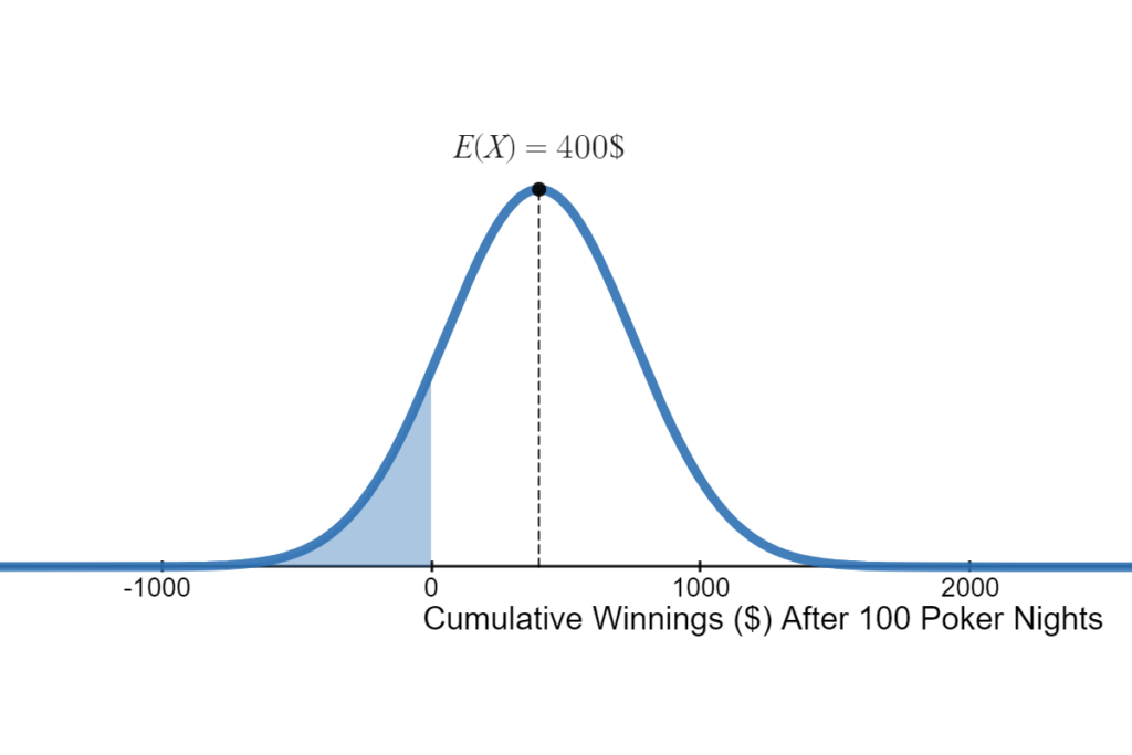
The blue area under the curve on the left of zero represents the probability of losing money after 100 poker nights, Given our parameters, I have approximately a 13% of losing money over the next 100 poker nights even though I’m a winning player!

Going Broke
What is the probability of going broke at any point, given a bankroll of a specific size?
To answer this question, I have simulated 10 000 instances of playing 100 poker nights given my win probabilities (R code). Below are just 10 instances to declutter the plot.
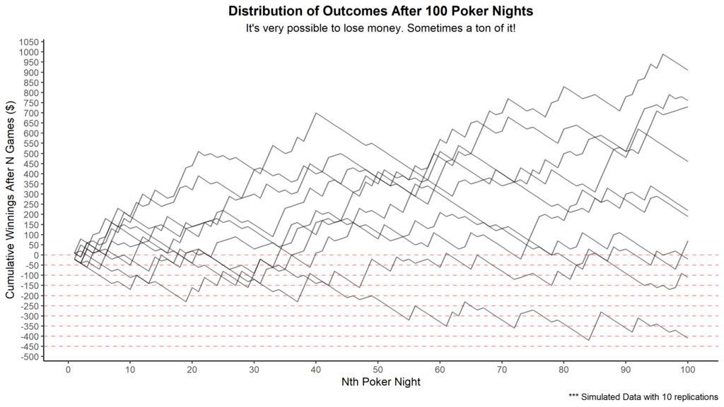
The endpoints of each line represent the net profit after 100 games. As you can see, most endpoints are above zero. This makes sense given that there’s approximately a 13% chance of losing money after 100 poker nights. That said, any line that dips below the horizontal line at -50$ represents a player that would have gone broke if they had a 50$ bankroll. The lowest jagged line represents an instance of going broke with a 400$ bankroll after playing around 85 poker nights. You may think that this is extremely unlikely and that it’d never happen to you. The fact is, you can expect to go broke about 3% of the time with a bankroll of 400$ despite being a great poker player relative to your peers.
Now let’s plot all 10 000 instances of playing 100 poker nights to see the full distribution and estimate some probabilities.
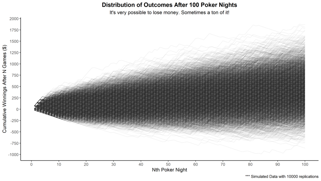
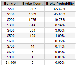
Many jagged lines end in the negatives, or at least were negative at some point along their journey. Another way to represent the endpoints of each line is with the histogram below.

There were 6567 jagged lines that dipped below 50$ at some point. In other words, roughly 2 players out of 3 with a bankroll of 50$ went bust in our sample. This is a ridiculously high rate of ruin. A more conservative bankroll would be wise to ensure that our skill level (signal) will have enough games to dominate the noise.
Bankroll Management
How big of a bankroll do we need to be 99% sure of not going broke?
A bankroll of roughly 500$ (25 buy-ins) was necessary to ensure a 99\% chance of not going broke, despite my skill level at 20$ buy-ins poker nights.
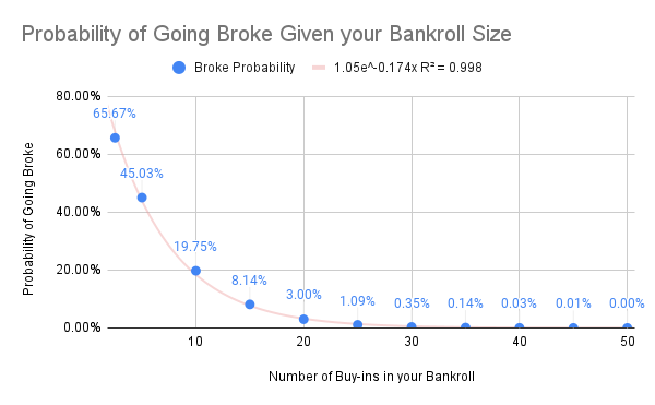
We can use the exponential curve that we obtain from Google Sheets to create the Desmos visualization below.
The point of intersection of the horizontal line and the curve represents the number of buy-ins it requires to guarantee a certain level of confidence of not going broke.
Final Thoughts
I hope that this article convinced you that a conservative risk-management strategy can be a superpower when it comes to long-term ventures. It’s only by playing it safe that we can afford to take on huge calculated risks for big payoffs. You can’t double your money if you’re broke!
Read This Next!
- Gambling versus Calculated Risk-Taking
- Catan Analytics: How to win with data-driven strategies
- What I Learned from Tracking my Mood for 1000 Days
- The Biggest Bluff – Book Notes
- Is it Luck or is it Skill?
- Life Score: A Subjectively Objective Way to Evaluate your Life
- Who’s the Best at Flipping Coins?
- Automate Your Finances
- The 300 000$ Meeting
- The Biometrics of High School Teaching
- The Relation between Phone Usage and Mood
- The Visual Display of Quantitative Information by Edward R. Tufte (2nd Edition)