Statistical Rethinking 2023 Notes

Takeaways (TLDR)

• Should include competing causes even if they aren’t confounds.
• Blindly adding all the variables in a model is foolish and often wrong.
• The causes cannot be found in the data. No causes in, no causes out. Cannot offload subjective responsibility to objective procedures.
• DAGs are the typical way to encode scientific knowledge (see DAGitty software).
• A causal effect is defined in terms of interventions.
• Steps to draw the Bayesian Owl:
  1. Theoretical estimand
  2. Scientific (causal) model(s)
  3. Use (1) & (2) to build statistical model(s)
  4. Simulate from (2) to validate (3) yields (1)
  5. Analyze real data
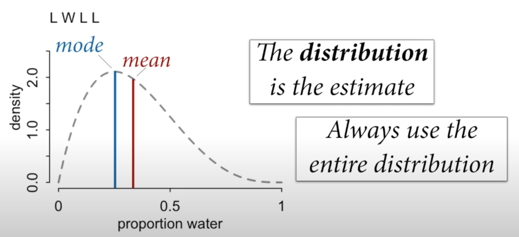
• In Bayesian inference, all estimates are posterior distributions. We can report a point, but that choice is arbitrary. It’s much better to report the entire distribution or the contrasts.
• Use priors that you can defend. Flat priors are rarely the best solution. Think about this as encoding another layer of scientific knowledge into the analysis.
• Simulation with Markov Chain Monte Carlo is a powerful technique.
• We can include measurement error and unobserved variables in our scientific model and perform sensitivity analysis to increase the validity of our results.
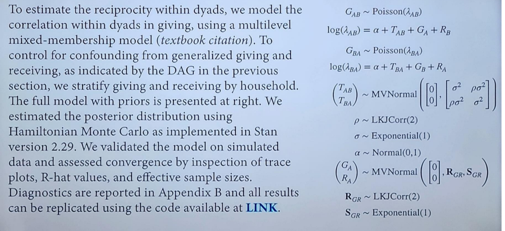
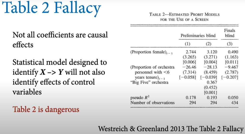
• Beware of the Table 2 Fallacy.

---

• YouTube lectures 2023 & Github repository
• Rethinking package

2023 – 01 – The Golem of Prague (Link)

• DAGs
  • Directed Acyclic Graphs
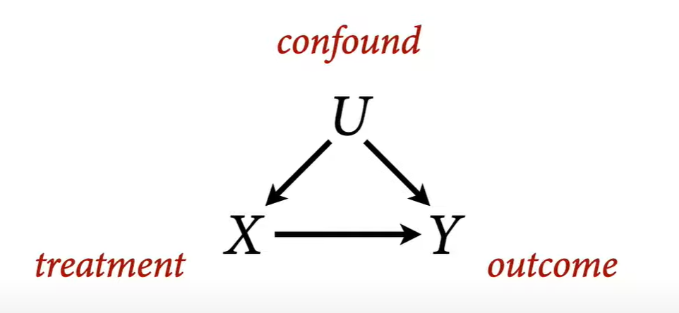
  • “No causes in, no causes out.”
  • Transparent scientific assumptions that connect theory to golems and exposes ourselves to productive critique.
  • Book of Why by Judea Pearl – Book Summary
• Golems:
  • Mindless statistical models.
  • Powerful yet dangerous.

• Owls:
  • Step 1: Draw an oval for the body. Step 2: Draw a circle for the head. Step 3: Draw the rest of the owl.
  • Communicate all intermediate steps of analysis.
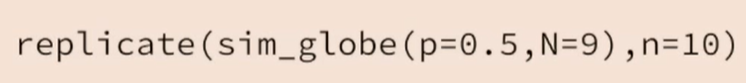
  • Use a scripting language to do your analysis. It creates reproducible research and aligns with open science.
  • Steps to draw the Bayesian Owl:
    1. Theoretical estimand
    2. Scientific (causal) model(s)
    3. Use (1) & (2) to build statistical model(s)
    4. Simulate from (2) to validate (3) yields (1)
    5. Analyze real data

Lecture 2 – The Garden of Forking Data

Bayesian Analysis

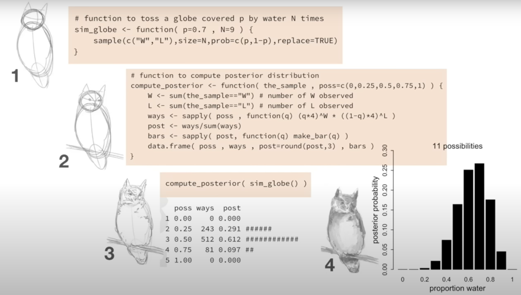
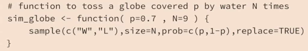
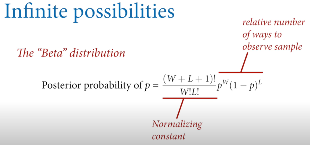
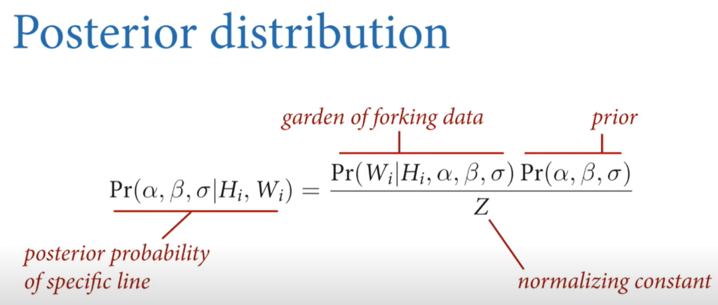
For each possible explanation of the sample, count all the ways the sample could happen.
Explanations with more ways to produce the sample are more plausible.

Bayesian Data Analysis

• Things that can happen in more ways are more plausible.
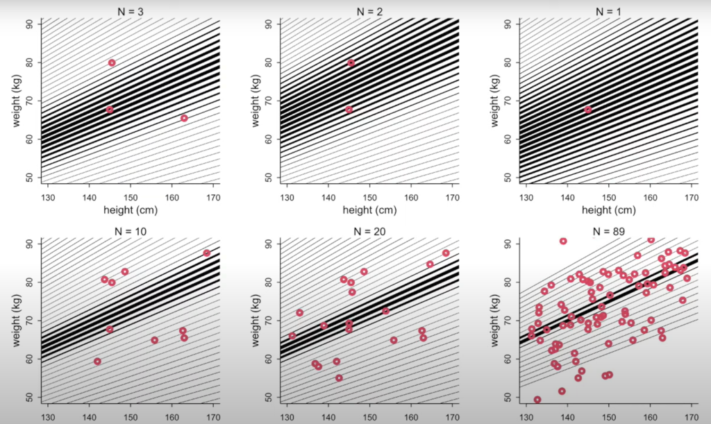
• The minimal sample size is 1 observation.
• The shape of the posterior distribution embodies the sample size.
• The estimate is a distribution, you can communicate the mode, mean, or median.
• No special intervals.

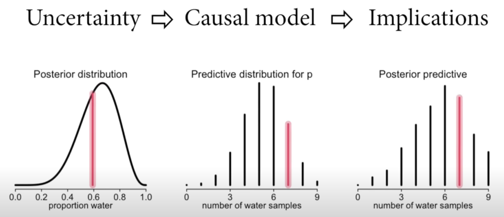
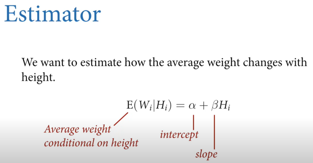
Workflow: What proportion of the globe is covered by land.

Step 1: Define a generative model of the sample. (DAG)

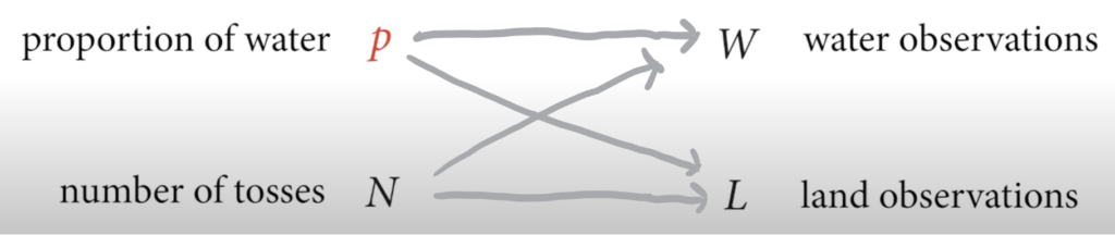
Step 2: Define a specific estimand.

Step 3: Design a statistical way to produce an estimate.

Step 4: Test (3) using (1).

• Test before you Est (imate).

Step 5: Analyze the sample & summarize.

• Sample from the

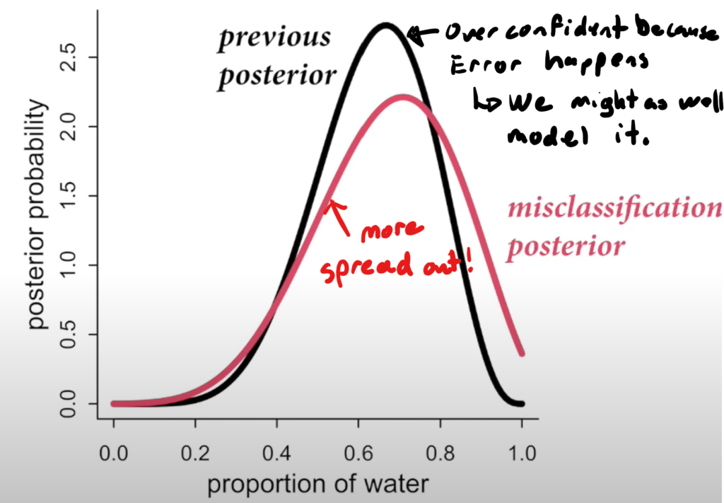
Misclassification & Measurement error

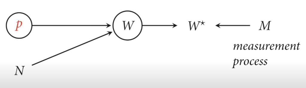
• Circles means unobserved variable.
• W* represents the misclassified samples that happen 10% of the time.

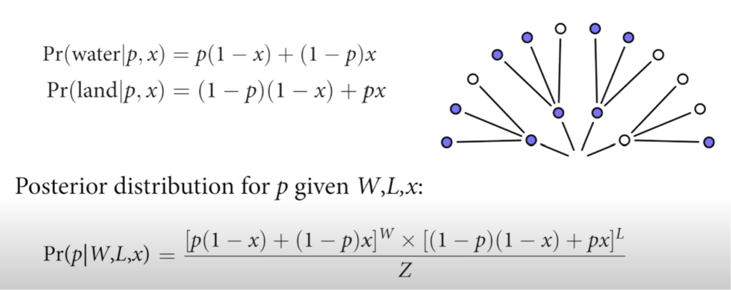
• P(water | p, x) = (water & True) Or (land & Misclassified)
• Measurement error, missing data, sample bias happen all the time. You might as well model it to have better estimations.
  • Creating a causal model of how the sampling process occurs for a survey, for example, can allow us to unbias the sample and provide good estimates for the population.

Lecture 3 – Geocentric Models

Drawing the Owl

1. Question/goal/estimand
2. Scientific model
3. Statistical model(s)
4. Validate model
5. Analyze data

Always stay in Flow. You don’t need to understand everything at all times. Design optimal challenges and keep moving forward. Learning is the goal. Not ultimate knowledge.

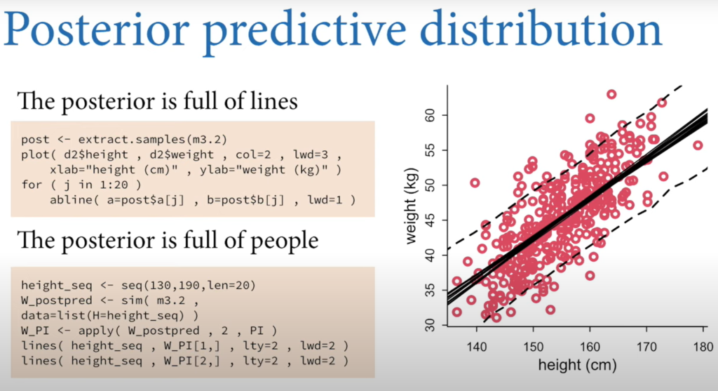
• Awesome animation of Bayesian estimation of line parameters.

Priors

• There are no correct priors, only scientifically justifiable priors.
• Don’t let your prior distribution allow nonsensical values.
• Priors should express scientific knowledge, but softly.
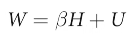
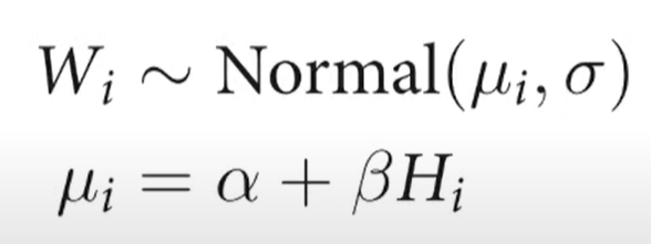
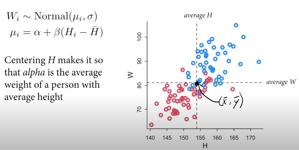
  • The intercept averages to zero. 0 cm tall and weighs 0 kg.
    • Alpha ~ N(0,10)
  • We know that weight increases with height. We also know that the weight in kilos is usually less than the height in cm.
    • Beta ~ U(0,1)
  • The standard deviation is always positive and less than 10 based on our expertise knowledge.
    • sigma ~ U(0, 10)
• The quap function is in the rethinking package.

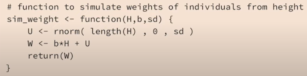
Prior Predictive Simulation

• This is what the Golem sees before seeing the data.

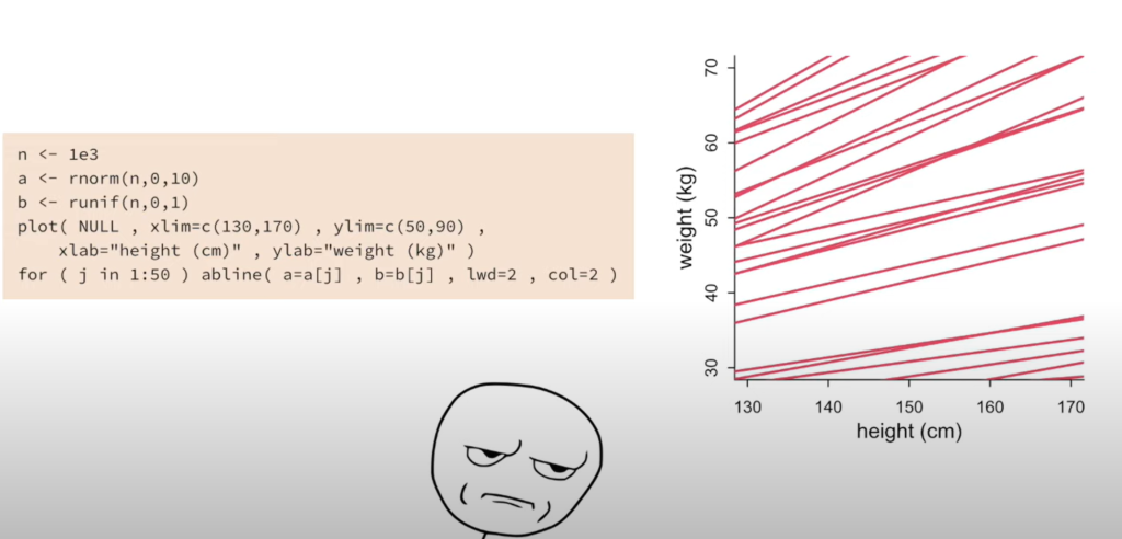
• Always test the model on simulated data! Before using the real data.
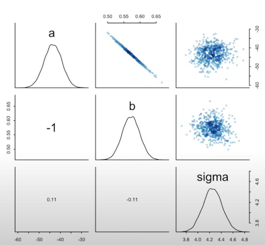
• Parameters are not independent!
• There is no one line of best fit in Bayesian analysis. Instead, there is only distributions of parameters.

Lecture 4 – Categories & Curves

Indicator variables

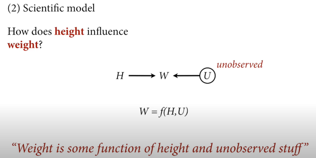
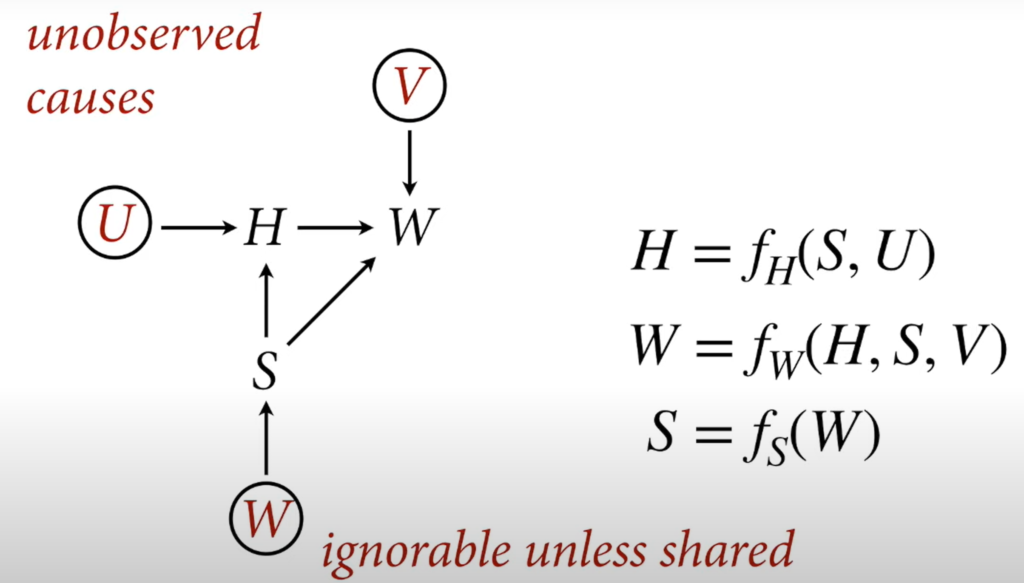
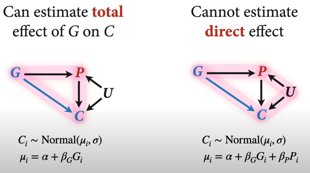
• Can ignore unobserved causes unless they are shared. We need to include confounders in our model to stratify by the confounder.
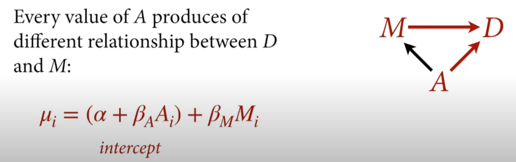
  • We should probably include nutrition here as it contributes to both height and weight.
  • We should also include age as it “causes” both Height and weight.

• Use index variables instead of indicator/dummy variables when creating factor variables by hand.
• Overlap of distributions does not indicate that variables don’t differ or that they do. We have to compute the contrasts.

We want to take the mean of the differences (using contrasts) and not the difference of the means. Don’t summarize then subtract. Subtract then summarize.

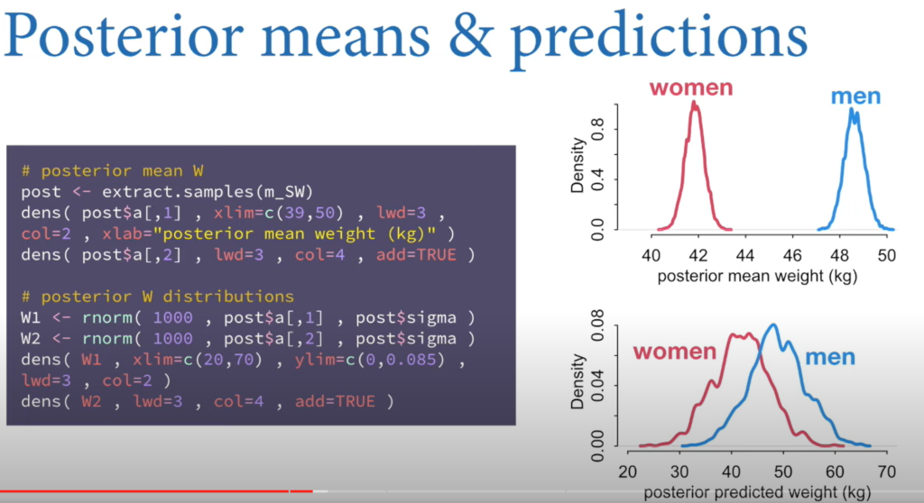
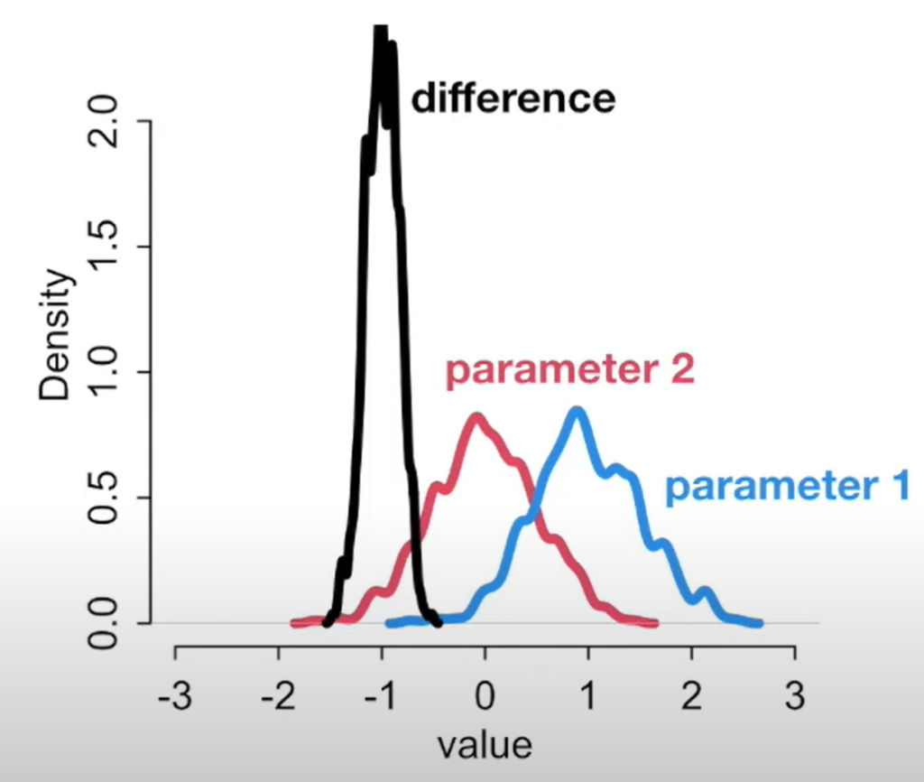
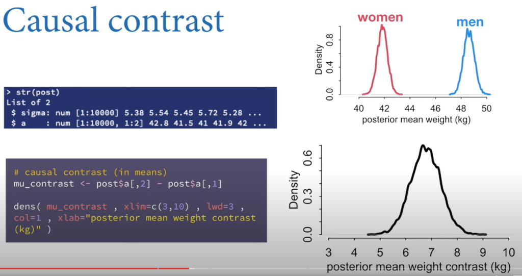
• You can compute the contrasts by subtracting the distributions.
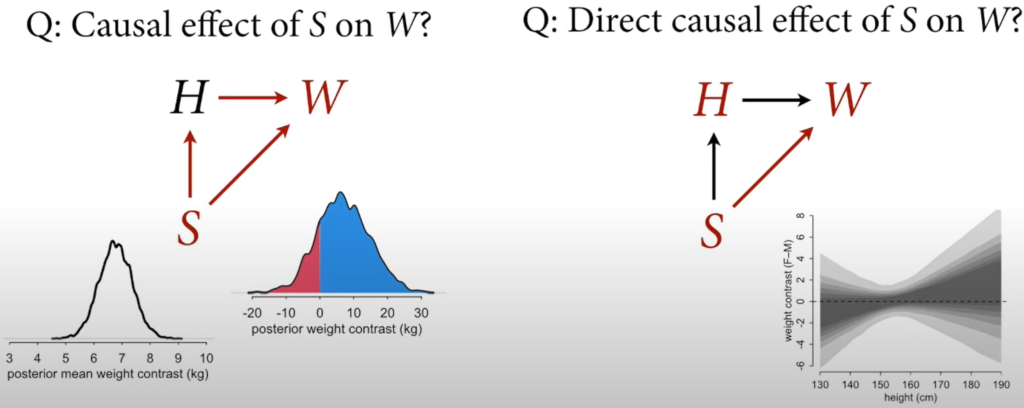
• If you select a man and a woman at random, 82% of the time, the man will be heavier.
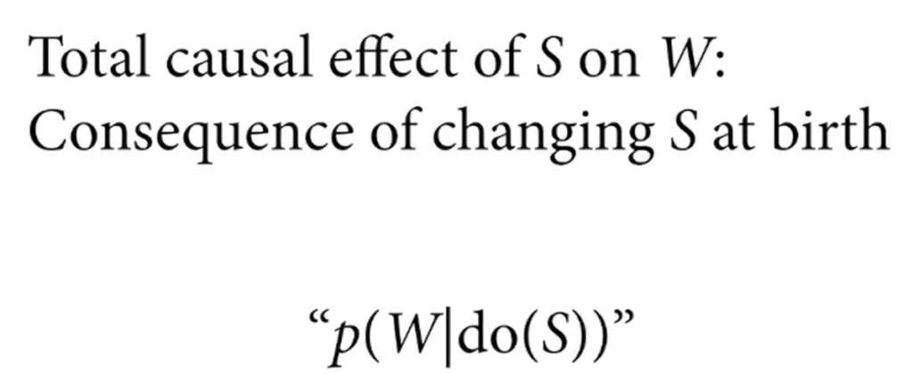
• The causal effect of S on W is the entire posterior distribution of contrasts.

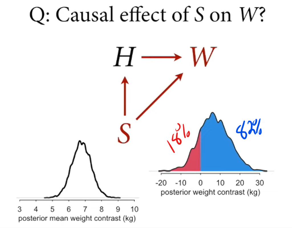
• To calculate the direct effect of Sex on Weight, you fit two regression lines for each sex and subtract the predicted weights for each height using the y values of the regression line.

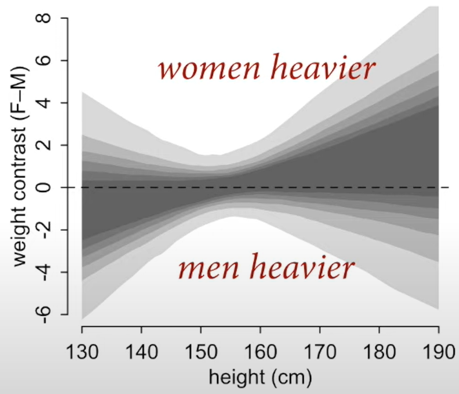
Since the centre of mass is near zero, you can say that the direct causal effect of sex on weight is minimal. Almost all the causal effect of Sex on Weight happens indirectly through height.

Curves from lines

• Don’t use polynomials. Splines are less bad.
  1. Reason: points anywhere on the x-axis, determine the equation of the entire parabola. There’s no local smoothing like with splines.
  2. Lots of uncertainty at the end ranges.

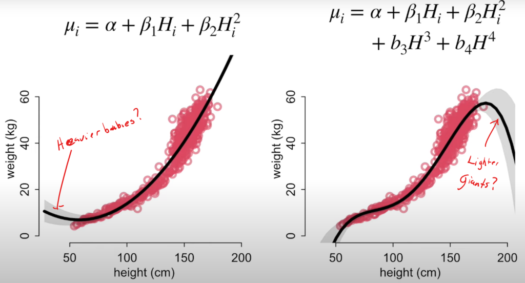
• Splines can fit anything but are not scientifically informed.
  • We know there are growth phases of life. It’d make more sense to model those.

Lecture 5 – Elemental Confounds

www.dagitty.net

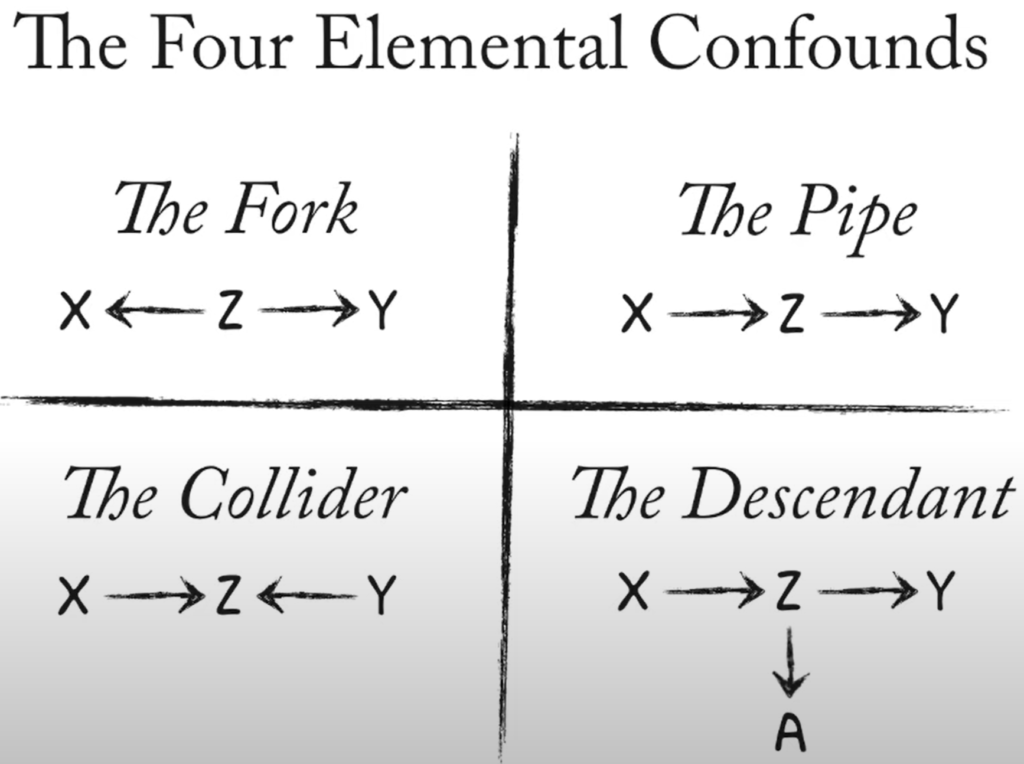
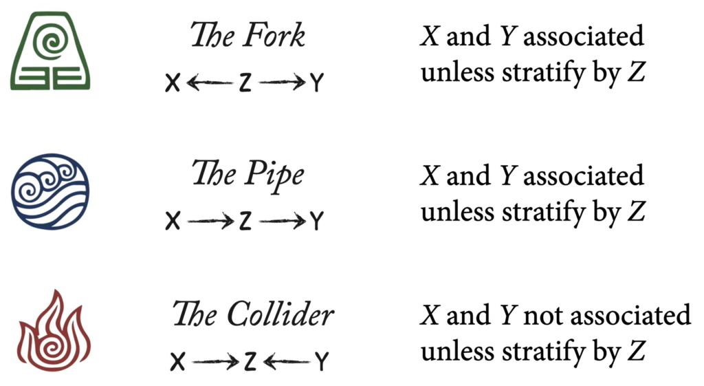
A Crash Course in Good and Bad Controls

Fork Flows, Collider closed, Pipe flows.

The Fork: X ⇽ Z ⇾ y

Controlling for a confound means stratifying a variable to see if correlation persists.

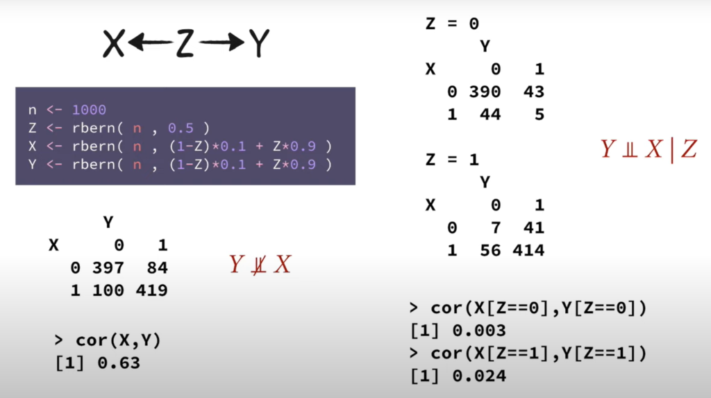
• What does it mean to stratify for a continuous variable?
  • Holding everything else constant.
• It’s always a good idea to standardize continuous variables.
• It’s not because zero is in an interval that an estimate is zero. The intervals are arbitrary.

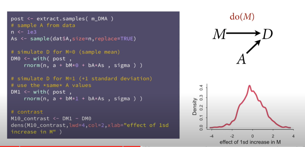
The causal effect of M on D. Intervene on M (delete all arrows going into M).

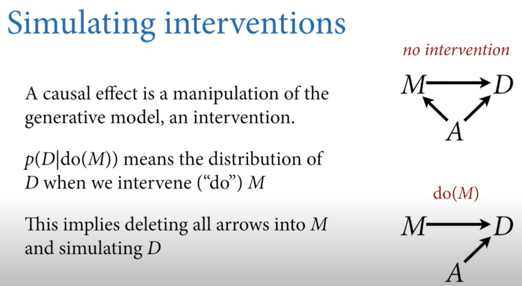
The intervention is to increase M to 1 standard deviation above the mean.

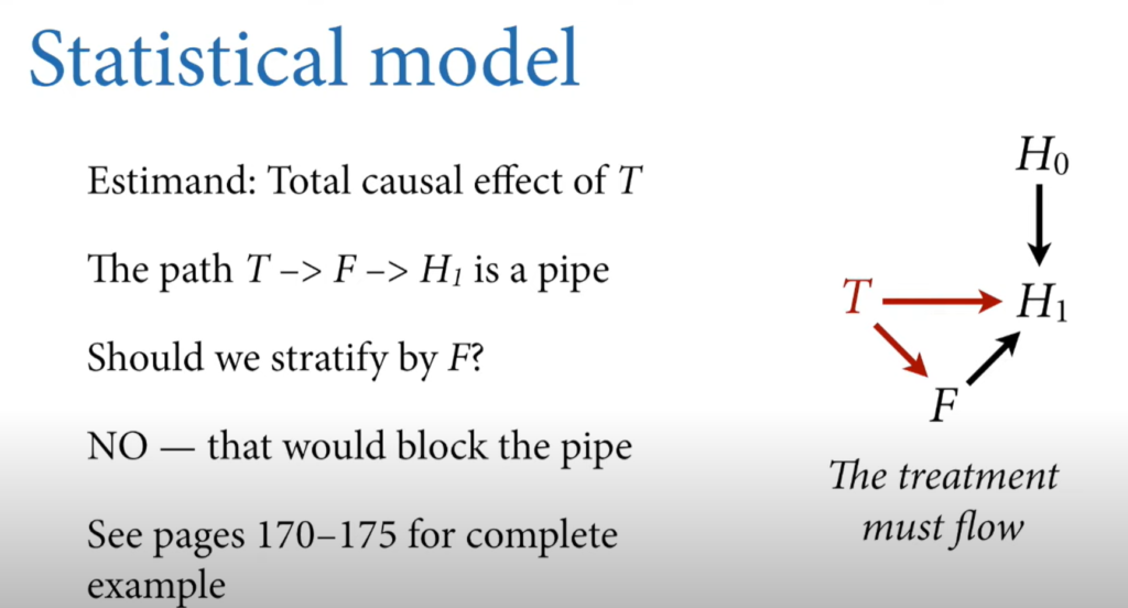
The Pipe (Mediator): X ⇾ Z ⇾Y

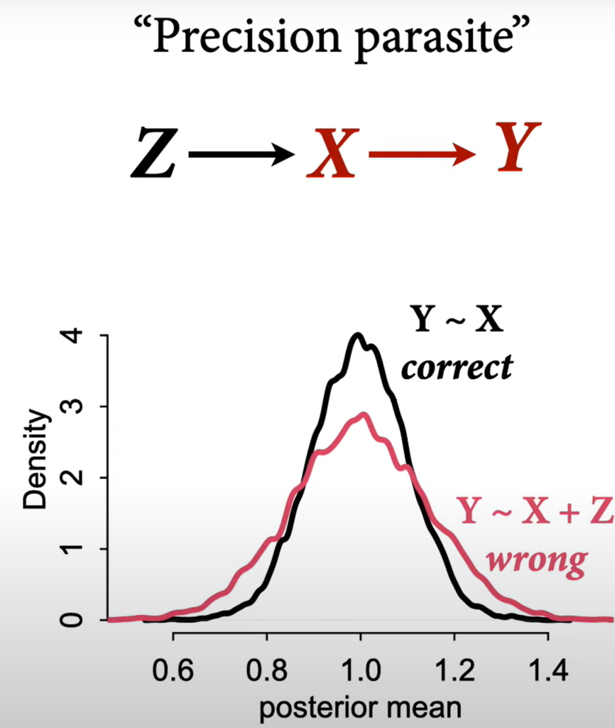
Don’t control for a mediator if looking for a total causal effect. Only control if looking for direct effect.

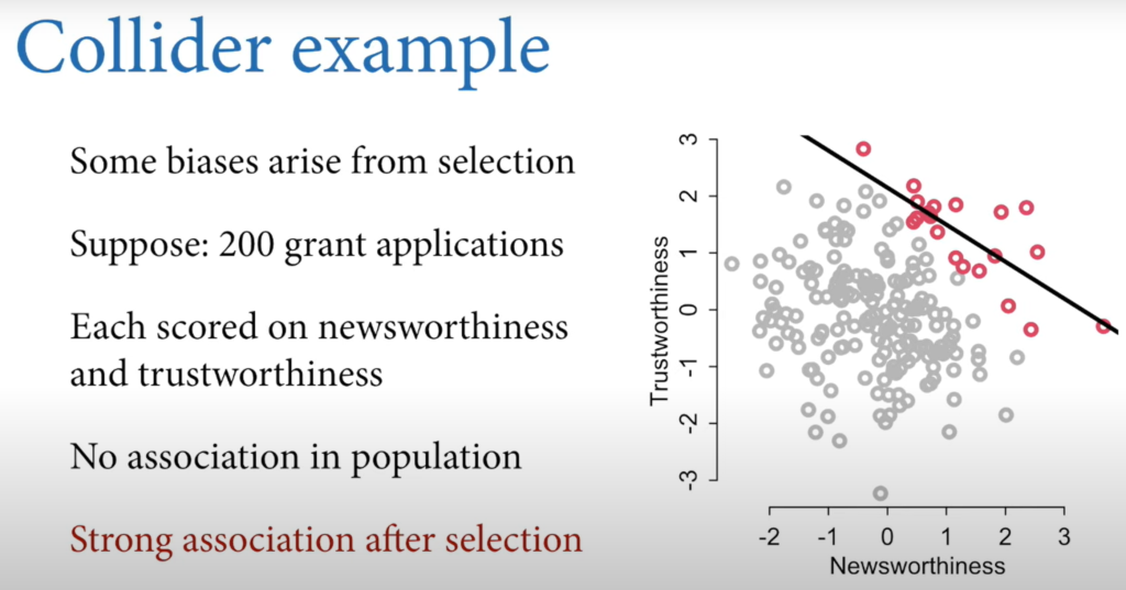
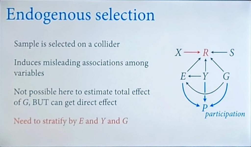
The Collider: X ⇾ Z ⇽ Y

Also known as selection bias.

• All jerks are hot
• No bad food in bad locations so we think bad neighbourhoods lead to good restaurants.

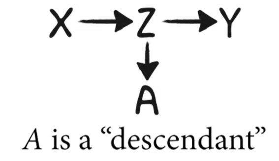
The Descendant

Lecture 6 – Good & Bad Controls

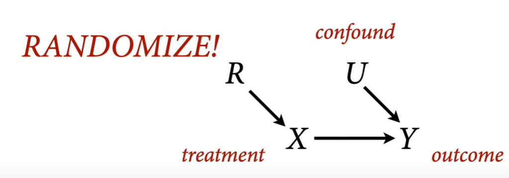
Randomization and intervention remove all arrows going into treatment variable.

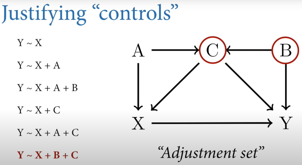
Backdoor Criterion

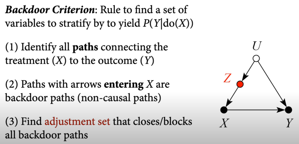
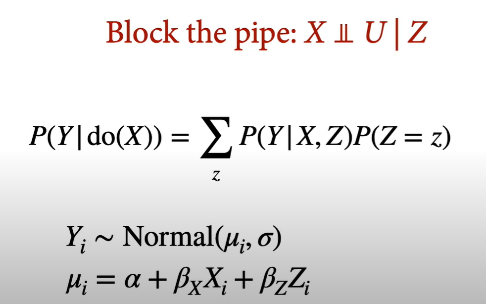
To block a pipe, stratify by the variable in the middle to block the flow.

Adjust by C and Z and Either A or B

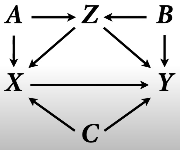
Don’t include Z in the model for both of these models. Second one is centered but too wide for nothing.

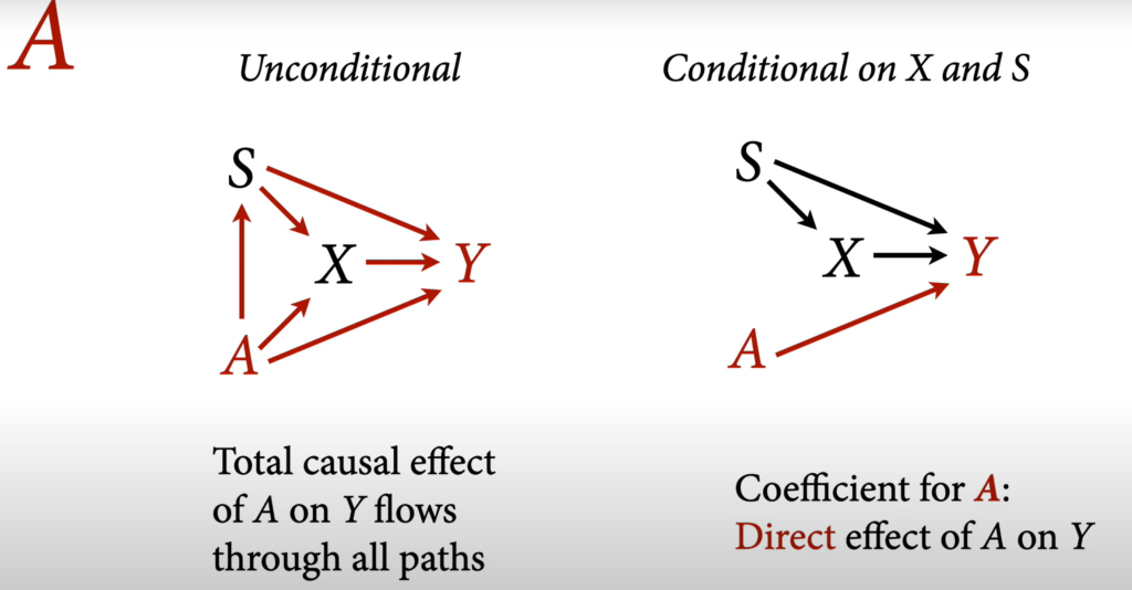
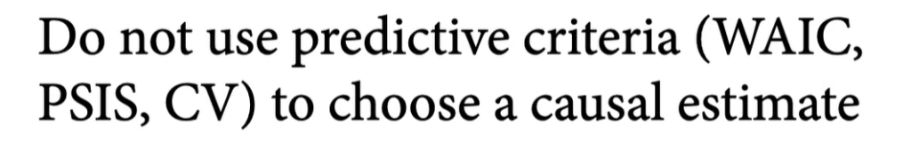
A table of coefficients should be avoided because not all coefficients represent direct causal effects.

The coefficients of S and A do NOT represent causal effects on y.

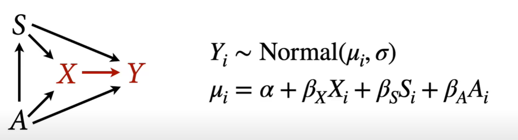
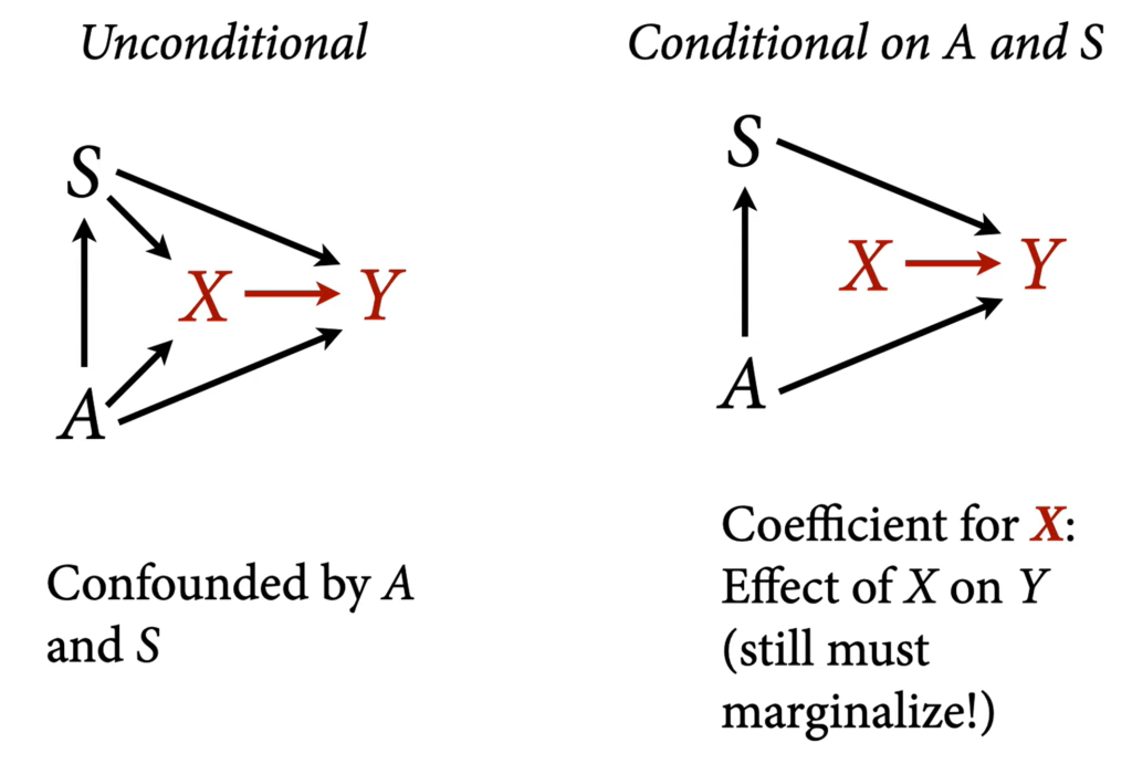
The difference between total causal effect and direct causal effect

Lecture 7 – Fitting Over & Under

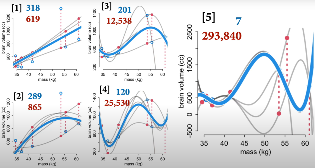
• Estimates are distributions. Points are decisions.
• In-sample error is lower with cubic and quadratic but way worse for out-of-sample error.

Regularization

To decrease overfitting, use skeptical priors (tight around zero).

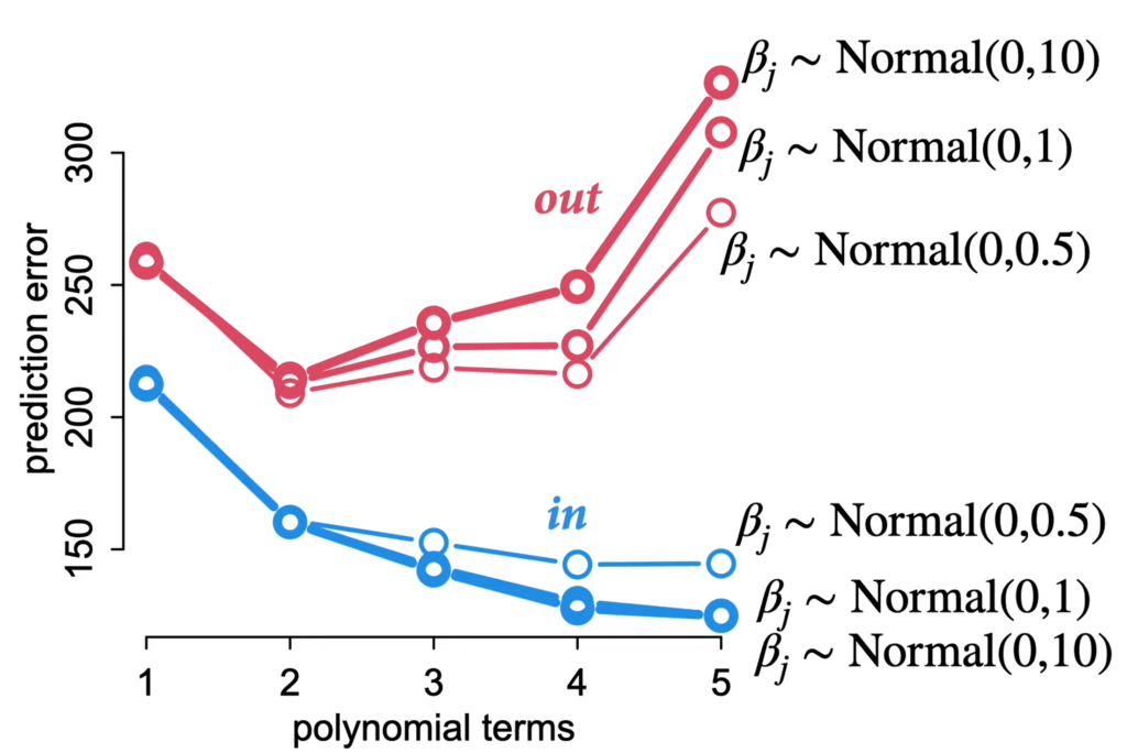
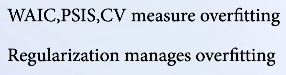
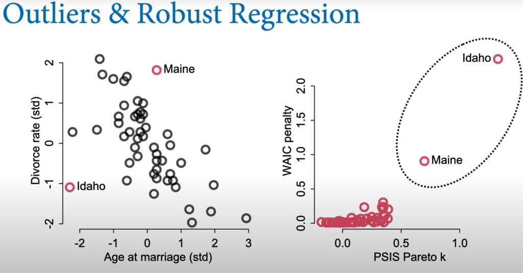
AIC is obsolete. Use WAIC instead. Richard prefers PSIS.

• For pure predictions without intervention, the models with confounds will do better.
• Deviance is essentially the error. Big numbers are bad.

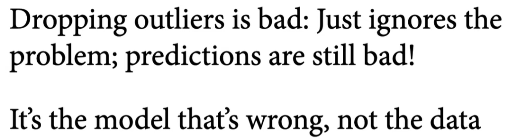
Use PSIS Pareto k and WAIC penalty to determine and quantify outliers.

Use t distribution (bigger tail) instead of normal to increase the robustness to outliers.

Lecture 8 – Markov Chain Monte Carlo

MCMC is the way to go to compute posteriors

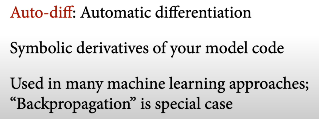
• You only need a few hundred samples to estimate the posterior. MCMC are efficient with gradients.

Lecture 9 – Modeling Events

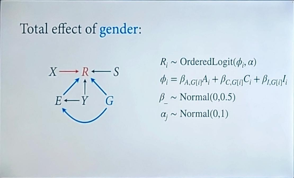
Discrimination

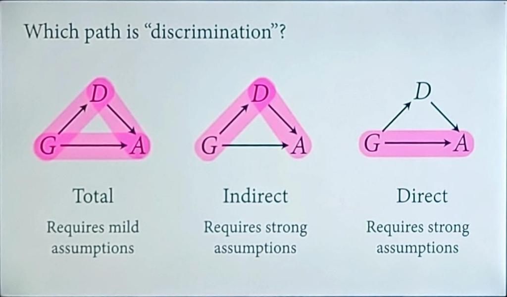
• Total: Experienced discrimination
• Indirect: Structural discrimination
• Direct: Status-based or taste-based discrimination
• To estimate the total causal effect of gender, we don’t stratify by department.
• To estimate direct effect of gender, we stratify by department.

Exponential Family

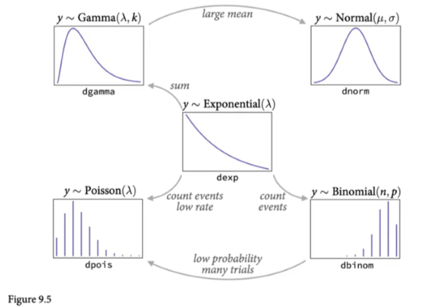
• Knowing which distribution to choose has to do with the constraints on the data.
• It’s not a good idea to test whether variables or normally distributed. Just assume and state your assumptions. You can’t test whether data are normally distributed.

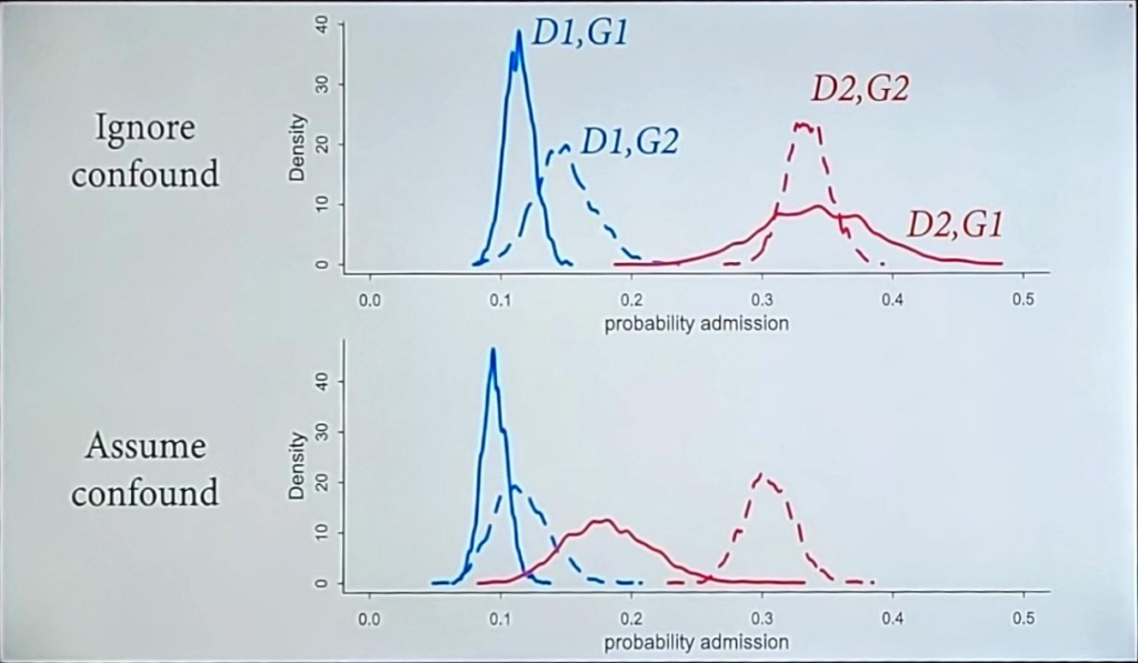
Lecture 10 – Counts & Hidden Confounds

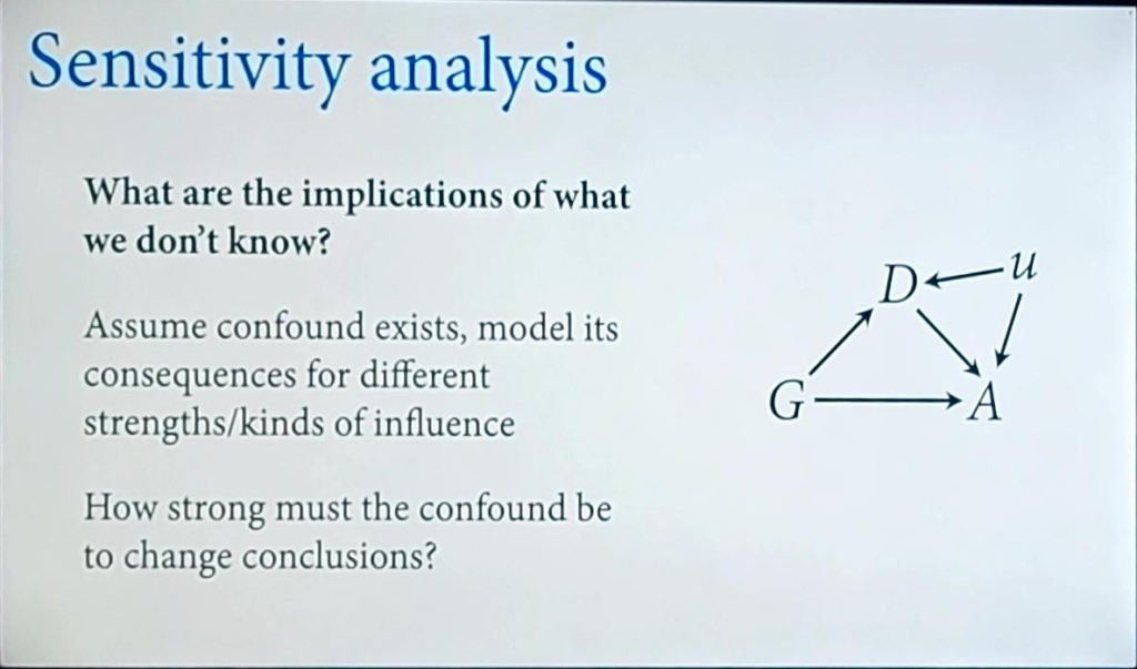
• Better than ignoring known confounds.
• What are the implications of what we don’t know?
• Vary the confound strength.

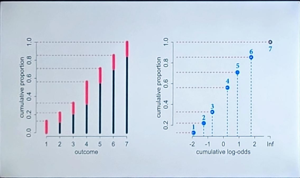
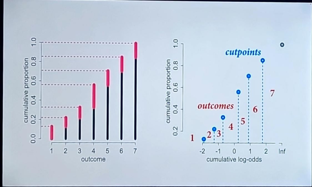
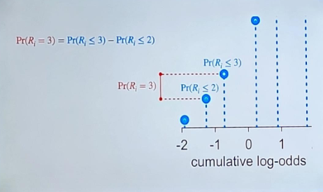
Lecture 11 – Ordered Categories

Convert frequency bar graph to cumulative frequency plot and then cumulative probability then cumulative log odds.

Should include competing causes even if they aren’t confounds.

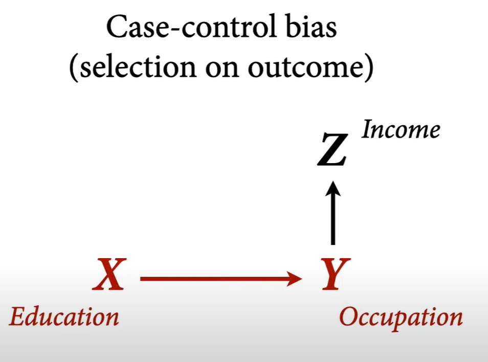
Participation bias

Lecture 12 –

Lecture 13 –

Lecture 14 –

Lecture 15 –

Lecture 16 –

Lecture 17 –

Lecture 18 –

Lecture 19 –

Lecture 20 – Horoscopes

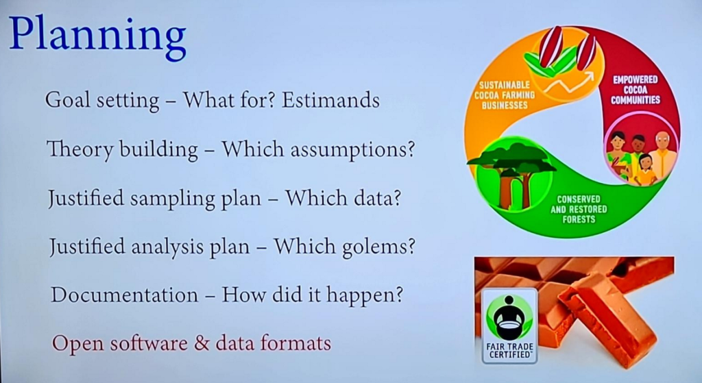
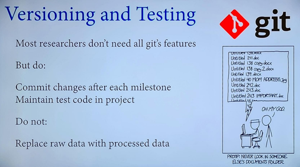
• It is unethical to use expensive software because the point of science is that others can inspect and try to replicate your results.
• The same can be said about data formats.
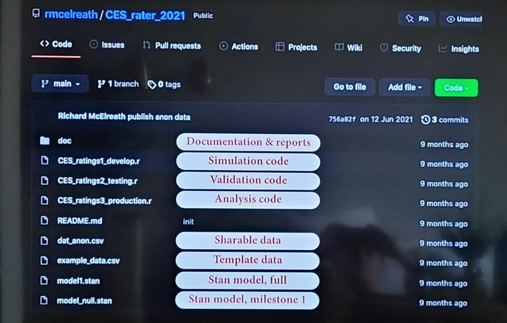
• Practice open science by posting your code on github with version control with comments.

• https://datacarpentry.org/
• Use code to process data. Save as csv file.
• Editing data in Excel is the equivalent of Pipestone by mouth.
• If you can’t share the actual data. Share a synthetic version.
• Cannot offload subjective responsibility to objective procedures.

Example of adequate communication: