I had a strange mathematical experience during my first year of teaching high school math. I gave my students a typical matching exercise to complete, like the one you see below.
| Item | Term | Definition |
| A | Variable | A relationship with a constant rate of change, forming a straight line graph. |
| B | Coefficient | A mathematical statement showing that two expressions are equal. |
| C | Linear Relationship | The amount of space inside a 2D shape, measured in square units. |
| D | Constant | A symbol (usually a letter) used to represent an unknown number or value. |
| E | Equation | The point where a line crosses the y-axis (when x = 0). |
| F | Slope | The average of a set of numbers, found by dividing the sum by how many there are. |
| G | Y-intercept | A number from 0 to 1 that shows how likely an event is to happen. |
| H | Area | A number multiplied by a variable in an algebraic expression (e.g., 3 in 3x). |
| I | Mean | The steepness of a line, calculated as rise over run (change in y over x). |
| J | Probability | A value that does not change in an expression or equation. |
It surprised me how much my students struggled on questions like these. A few students even managed to get zero correct matches! I was baffled. I thought that even a student who completely guesses at random is unlikely get zero right answers. Since I hold a statistics degree and teach statistics at my school, I set out to answer the following question.
What is the probability of getting zero right answers on a matching question with n items?
Drawing It Out
Let’s consider a question with three items only.
| Item | Term | Definition |
| A | Variable | A relationship with a constant rate of change, forming a straight line graph. |
| B | Coefficient | A symbol (usually a letter) used to represent an unknown number or value. |
| C | Linear Relationship | A number multiplied by a variable in an algebraic expression (e.g., 3 in 3x). |
There are six possible ways of matching the terms and definitions above. There are three options for the first term, two options for the second and one for the last term. Drawing the possibility tree is the best way to visualize all the arrangements.
![\[3\times 2 \times 1 = 6\]](https://duddhawork.com/wp-content/ql-cache/quicklatex.com-72ff5522e52ed6002c5587ccab4b3716_l3.png "Rendered by QuickLaTeX.com")
We can see that, in general, if we had  items, we’d have
  arrangements. Mathematicians came up with the factorial notation
  to represent this concept.
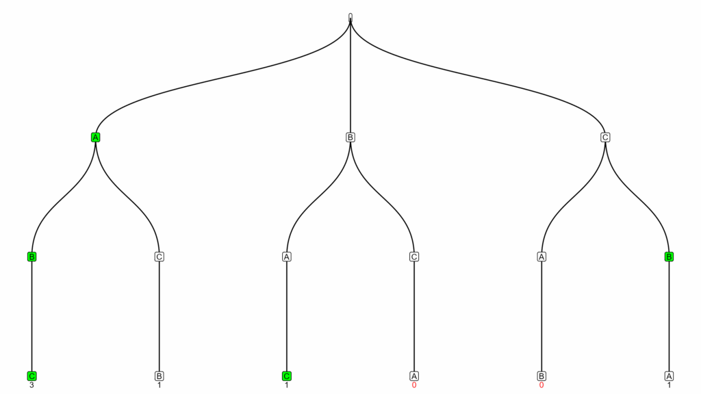
The six arrangements are ABC, ACB, BAC, BCA, CAB, and CBA. The right answers are plotted in green, and the number of correct answers for each arrangement is indicated below each branch. We see that there’s only one way to get all the right answers. Additionally, it’s impossible to get  correct answers because the last option will be good if all the others were correct.
| # of Correct Answers | # of Arrangements | Probability |
| 0 | 2 | 33% |
| 1 | 3 | 50% |
| 2 | 0 | 0% |
| 3 | 1 | 17% |
| TOTAL | 6 | 100% |
What is the probability of getting zero right answers on a matching question with 3 items?
Sometimes the best way to answer a difficult question is to start by answering similar, but simpler one. We see that, when guessing at random, the probability of getting zero right answers on a matching question with 3 items is  %.
%.
Let’s repeat this process for four items to build our intuition.
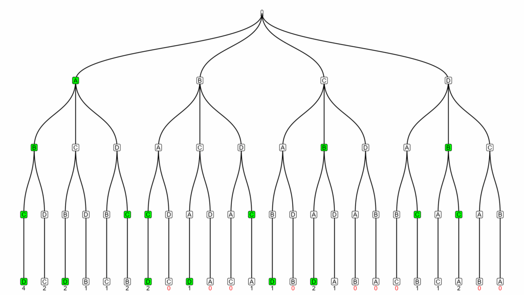
There are now  possible ways of arranging four items.
| # of Correct Answers | # of Arrangements | Probability |
| 0 | 9 | 38% |
| 1 | 8 | 33% |
| 2 | 6 | 25% |
| 3 | 0 | 0% |
| 4 | 1 | 4% |
| TOTAL | 24 | 100% |
We see that there is still only one way to get all the correct answers. The probability of getting zero right answers moved from 33% to 38%.
The factorial function grows fast. Ten factorial is over three million.
| n | n! |
| 1 | 1 |
| 2 | 2 |
| 3 | 6 |
| 4 | 24 |
| 5 | 120 |
| 6 | 720 |
| 7 | 5,040 |
| 8 | 40,320 |
| 9 | 365,880 |
| 10 | 3,628,800 |
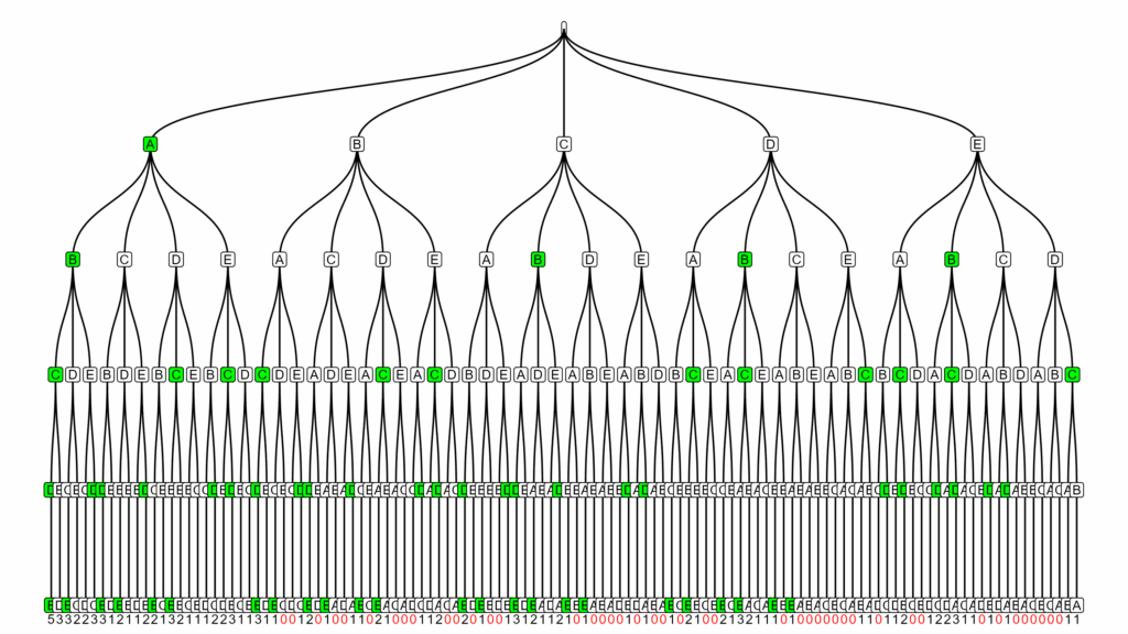
For this reason, we’ll only plot the tree with five items. We’ll use computer programming to determine the probability for larger values of n.
| # of Correct Answers | # of Arrangements | Probability |
| 0 | 44 | 37% |
| 1 | 45 | 38% |
| 2 | 20 | 17% |
| 3 | 10 | 8% |
| 4 | 0 | 0% |
| 5 | 1 | 1% |
| TOTAL | 120 | 100% |
Surprisingly, the probability of getting zero right answers barely moved. It appears to approach a certain value as n increases. This is the result for larger numbers of items.
| n | # of Arrangements | n! | Probability |
| 2 | 1 | 2 | 50% |
| 3 | 2 | 6 | 33.3% |
| 4 | 9 | 24 | 37.5% |
| 5 | 44 | 120 | 36.7% |
| 6 | 265 | 720 | 36.8% |
| 7 | 1854 | 5,040 | 36.8% |
| 8 | 14833 | 40,320 | 36.8% |
| 9 | 133496 | 365,880 | 36.8% |
| 10 | 1334961 | 3,628,800 | 36.8% |
The probability seems to stabilize around 0.368. I find it easier to see what is going on by plotting the numbers in the table.
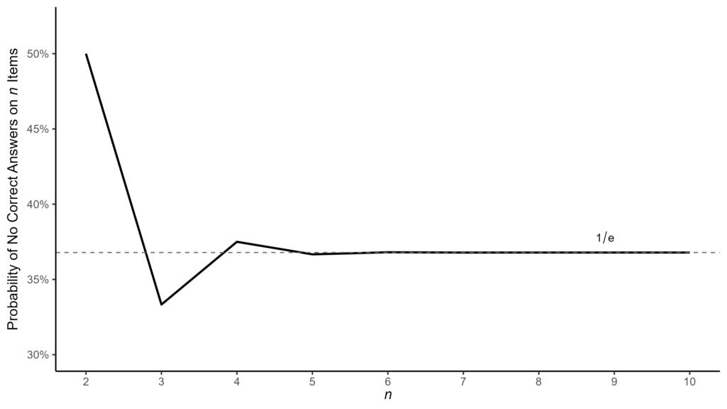
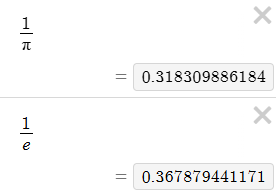
Something special happens when things converge to a specific number in mathematics. The first special number I could think of was  . Unfortunately, this is nowhere near our value of 0.368. So I had the idea of dividing one by Pi, which gave me 0.318. So close but not close enough.
Another famous constant in mathematics is Euler’s number  . Again, dividing one by
  gives us… drum roll… 0.368!!!!!!!!!!!!!!!
Note: The exclamation marks above are not factorials. 😋
This was one of the most awe-inspiring moments of my mathematical career. I set out to calculate a probability about my students, and then shows up seemingly out of nowhere. I felt like how the ancient mathematicians must have felt when they discovered that the ratio of a circle’s circumference to its diameter is the same number for all circles.
Mathematical Proof
It’s cool that we were able to use computers and intuition to show that the probability of getting no correct answers approaches  as the number of questions increases. However, ideally, we’d show mathematically that
![\[\lim_{n \to \infty} \frac{D_n}{n!} = \frac{1}{e}\]](https://duddhawork.com/wp-content/ql-cache/quicklatex.com-1edd035cecbf59cd1e86f04e520eb9e2_l3.png "Rendered by QuickLaTeX.com")
where  is the number of ways to get zero right answers and is the number of items. To do so, we need to determine the mathematical function that relates the number of items and the number of ways it’s possible to get zero correct answers.
| n | # of Arrangements (D_n) |
| 2 | 1 |
| 3 | 2 |
| 4 | 9 |
| 5 | 44 |
| 6 | 265 |
| 7 | 1854 |
| 8 | 14833 |
| 9 | 133496 |
| 10 | 1334961 |
The function is
![\[D_n = n! \sum_{k=0}^n \frac{(-1)^k}{k!}\]](https://duddhawork.com/wp-content/ql-cache/quicklatex.com-41392c4cc200417d40ccf4cc49c609bf_l3.png "Rendered by QuickLaTeX.com")
It turns out this formula has a name. represents the number of derangements and is sometimes denoted as  .
.
A derangement is a permutation of the elements of a set in which no element appears in its original position.
Wikipedia
Let’s try a few values of .
![\[D_2 = 2! \sum_{k=0}^2 \frac{(-1)^k}{k!} = (2 \times 1) \times \left[\frac{(-1)^0}{0!} + \frac{(-1)^1}{1!} + \frac{(-1)^2}{2!} \right] = 2 \times \left[1 + -1 + \frac{1}{2} \right]\]](https://duddhawork.com/wp-content/ql-cache/quicklatex.com-cf0d4a455861ea3e31cc46369c29c9dd_l3.png "Rendered by QuickLaTeX.com")
![\[D_3 = 3! \sum_{k=0}^3 \frac{(-1)^k}{k!} = (3 \times 2 \times 1) \times \left[\frac{(-1)^0}{0!} + \frac{(-1)^1}{1!} + \frac{(-1)^2}{2!} + \frac{(-1)^3}{3!} \right] = 6 \times \left[1 + -1 + \frac{1}{2} + \frac{-1}{6} \right] = 6 \times \left[ \frac{3}{6} - \frac{1}{6} \right] = 2\]](https://duddhawork.com/wp-content/ql-cache/quicklatex.com-43a18e0974245fe5dccbf897538a13ca_l3.png "Rendered by QuickLaTeX.com")
![\[D_5 = 5! \sum_{k=0}^5 \frac{(-1)^k}{k!} = 120 \times \left[\frac{1}{3} + \frac{(-1)^4}{4!} + \frac{(-1)^5}{5!} \right] = 120 \times \left[\frac{1}{3} + \frac{1}{24} + \frac{-1}{120} \right] = 120 \times \left[\frac{44}{120} \right] = 44\]](https://duddhawork.com/wp-content/ql-cache/quicklatex.com-19f5d56c23227d00ab3cb33f9206dcca_l3.png "Rendered by QuickLaTeX.com")
Nice! We’ve shown that  (at least for three examples).
Let’s substitute this function into our initial equation.
![\[\lim_{n \to \infty} \frac{D_n}{n!} = \lim_{n \to \infty} \frac{n! \sum_{k=0}^n \frac{(-1)^k}{k!}}{n!}\]](https://duddhawork.com/wp-content/ql-cache/quicklatex.com-102c742b7cb5187977e74c427f12266f_l3.png "Rendered by QuickLaTeX.com")
Cancelling out the on the top and bottom gives us:
![\[\lim_{n \to \infty} \frac{D_n}{n!} = \lim_{n \to \infty} \sum_{k=0}^n \frac{(-1)^k}{k!}\]](https://duddhawork.com/wp-content/ql-cache/quicklatex.com-32f6289776fcdfa325c7fb6cedb1ad1f_l3.png "Rendered by QuickLaTeX.com")
Thus, we need to show that  .
.
Let’s start by showing something simpler first. Consider the following table where the last column is the cumulative sum of  .
.
| n | n! | 1 / n! | Cumulative Sum |
| 0 | 1 | 1 | 1 |
| 1 | 1 | 1 | 2 |
| 2 | 2 | 0.5 | 2.5 |
| 3 | 6 | 0.167 | 2.667 |
| 4 | 24 | 0.042 | 2.708 |
| 5 | 120 | 0.008 | 2.717 |
| 6 | 720 | 0.001 | 2.718 |
| 7 | 5,040 | 0.000 | 2.718 |
| 8 | 40,320 | 0.000 | 2.718 |
| 9 | 365,880 | 0.000 | 2.718 |
| 10 | 3,628,800 | 0.000 | 2.718 |
We see that the values in the last column approach Euler’s number . We can express this fact mathematically as :
![\[e = \sum_{k=0}^{\infty} \frac{1}{k!} \approx 2.718\]](https://duddhawork.com/wp-content/ql-cache/quicklatex.com-c66b24cdfff1f3b91660e02a5c2a20da_l3.png "Rendered by QuickLaTeX.com")
This is a special case of the Taylor series for  where
where
![\[e^x = \sum_{k=0}^{\infty} \frac{x^k}{k!}\]](https://duddhawork.com/wp-content/ql-cache/quicklatex.com-d50b57e9b57bb800bf0667e43852f1e7_l3.png "Rendered by QuickLaTeX.com")
Substituting  gives us the result above that
  . However, substituting
  gives us
![\[e^{-1} = \frac{1}{e} = \sum_{k=0}^{\infty} \frac{(-1)^k}{k!}\]](https://duddhawork.com/wp-content/ql-cache/quicklatex.com-f87d459e7d93ad7b78ea96bf3864bbdf_l3.png "Rendered by QuickLaTeX.com")
Thus, we have shown that .
The theory of derangements can be applied to the gift exchange custom of Secret Santa. The probability that no one picks their own name approaches as the number of people increases. As we’ve seen, it only takes about five people for the probability to be very close to the magic number of 0.368.
Read This Next
- Catan Analytics: How to win with data-driven strategies
- Does it Make Sense to Buy Raffle Tickets?
- Is it Luck or is it Skill?
- Is Sports Betting Worthwhile?
- Life Score: A Subjectively Objective Way to Evaluate your Life
- Who’s the Best at Flipping Coins?
- How To Think About Teaching
- How To Teach
- The Tutor & The Gardener – My Teaching Philosophy