3 Modeling Basketball Shots
Note that all the R code used in this book is accessible on GitHub.
Shot distance and shot angle can always be calculated given shot coordinates. Interesting insights can be generated from this augmented data.
3.1 Visusalizing our Data
3.1.1 Shot Distance
We can try to visualize the relationship between shot distance (feet) and the probability of making a shot based on our data set.
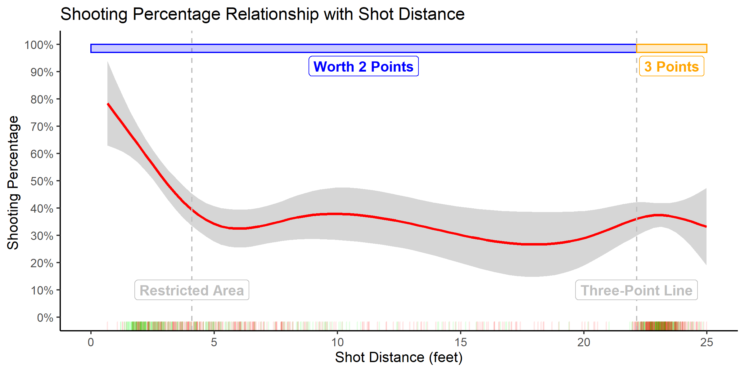
The accuracy starts off at approximately 75% for shots at the rim and levels off at 35% for shots further than 5 feet from the hoop. That's a drop in shooting percentage of roughly 40 percentage points between zero and five feet. Notice that the three-point shooting percentage is not much different from the mid-range accuracy.
This plot provides evidence for the hypothesis proposed in the first chapter. Attempts at the rim provide more expected points per shot than any other shot attempt. This is especially true considering that attackers tend to get fouled more often by attacking the rim.
An average team will make about 75% of their free throw attempts. Three quarters of two points is 1.5 points which is even better than the expected points of layups sitting at \(0.6 \times 2 ~\mbox{points} = 1.2\) expected points per shot. Furthermore, the average mid-range shot from our sample produced roughly \(0.35 \times 2 ~\mbox{points} = 0.7\) points per shot compared to \(0.35 \times 3 ~\mbox{points} = 1.05\) points per shot for the average three-point attempt. This implies that teams who evaluate their possessions through the lens of expected points should embrace the following hierarchy for possession quality:
\[ \mbox{2 or more free throws} > \mbox{lay up} > \mbox{3-pointer} > \mbox{mid-range} \] Of course, this strategy needs more nuance. Its implementation will depend on many factors such as the score of the game, who is on the court, the time remaining on the clock, and so on. Nevertheless, teams at the highest levels of the game have found success by reorienting their strategy to mirror this framework.
3.1.2 Shot Angle
We can also attempt to visualize how the angle from the center line of each shot affects shooting performance. Players often report that it is easier to shoot from the center of the court. Noah Basketball has also found that players taking three-point shots from the corners tended miss systematically away from the backboard (read the full paper here). This bias was stronger from the right-corner-three which was hypothesized to have something to do with the fact that most shooters are right-handed.
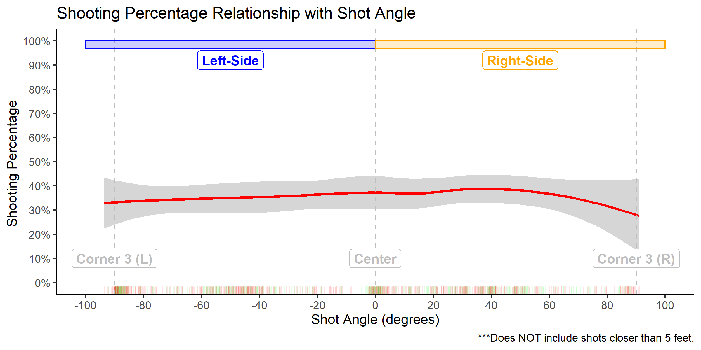
The shooting percentage for shots further than 5 ft does not seem to be affected by shot angle. Shots coming from the center do not seem to go in at a significantly higher rate than shots coming from the sides. There appears to be slight drop in shooting percentage for shots coming from the right (90 degrees) which could be evidence that supports NOAH's findings. However, this effect may not be robust enough to be statistically or practically significant. The rug distribution of shots located at the bottom of the graph indicates clusters at 0 degrees, 45 degrees, and 90 degrees. This makes sense given common basketball offensive strategies.
The previous plot showed no obvious differences between shooting from the left or right side of the court. We can take the absolute value of the shooting angle to essentially fold our graph in half. This allows us to narrow in on the effect of shooting angle on shooting percentage.
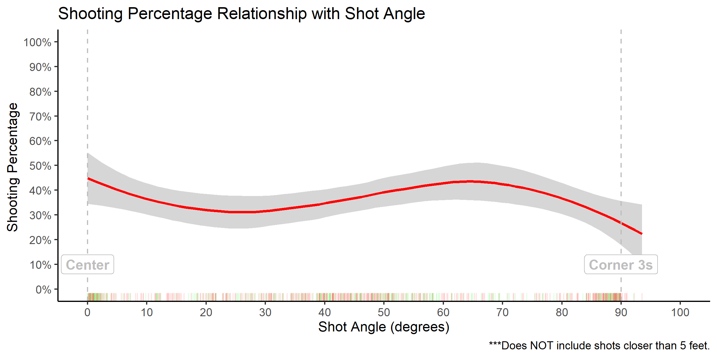
Taking the absolute value of the shooting angle reveals a different story. Attempts perpendicular to the center line (90 degrees) seem to have significantly lower accuracy than shots coming from the center. The relationship between shot angle and accuracy is not clear cut for our sample. More data may shed more insight.
3.1.3 Player
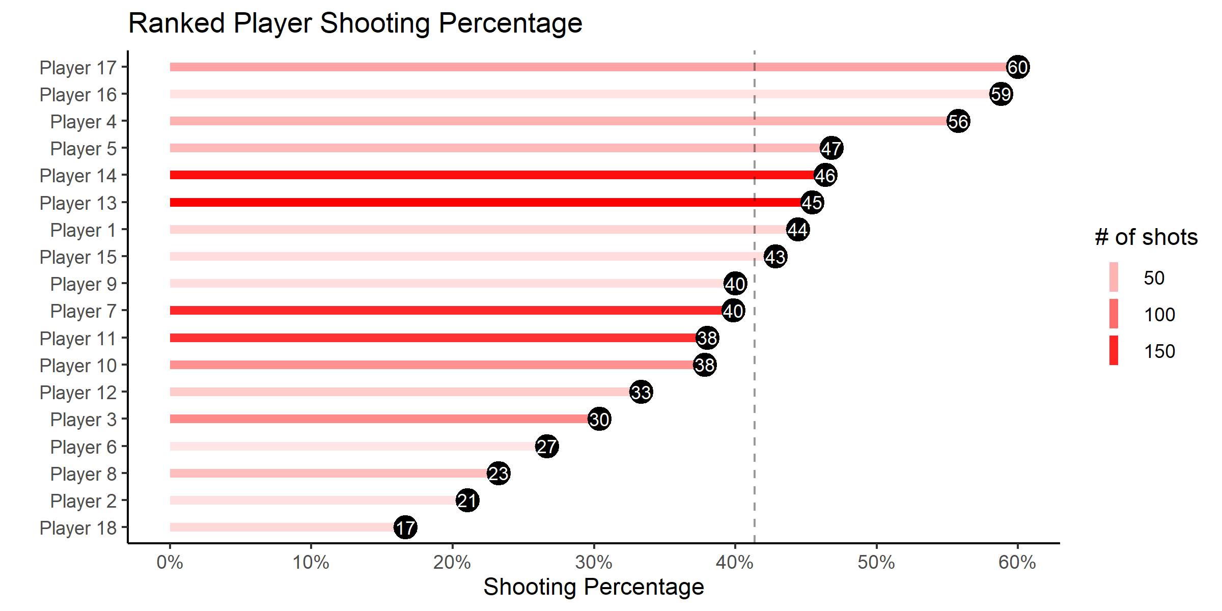
As you can see from the image above, some players seem to be shooting significantly better than others. Strictly looking at the field goal percentages can be misleading however. What if the most accurate shooter only took easy layups? We will see how we can try to separate shot ability from shot difficulty by modeling our data in the next section.
3.2 Quantifying these Effects
Pretty pictures are great. That said, they may struggle to display and quantify how different variables may interact. Technically, the red squiggle rom geom_smooth() in the pictures above used a model to predict the accuracy of the shooters for every distance. Let's try to model these effects more thoroughly.
3.2.1 Logistic Regression
Logistic regression is a machine learning tool used to model binary outcomes (made or missed shot in our case). We won't dive too deep into the modeling rabbit hole since the focus of this series of article is on the spatial analysis of basketball shots with an emphasis on visualizations.
We are trying the find the average shooter's probability of making a shot given a certain distance (measured in feet). Mathematically speaking, we can write this probability as:
\[ P(X) = P(Y = \mbox{Make} ~| ~ X = \mbox{distance}) \] We know that probabilities have to range between zero and one. The issue with using the classic linear regression model \(P(X) = \beta_0 + \beta_1X\) is that a straight line can give values higher than one or lower than zero (more on this below). To keep our probabilities between zero and one, we can use the logistic function.
\[ P(X) = \frac{e^{\beta_0 + \beta_1X}}{e^{\beta_0 + \beta_1X} + 1} \]
Note that exponentiating \(\beta_0 + \beta_1X\) removes the possibility of a negative probability. We also divide a positive number by a a greater positive number to keep our output below 1 (hence the \(+1\) in the denominator).
The logistic function can be rearrange in the following way:
\[ \log \left( \frac{P(X)}{1 - P(X)} \right) = \beta_0 + \beta_1X \] Note that we can easily switch back and forth between the log-odds \(\log \left( \frac{P(X)}{1 - P(X)} \right)\), the odds \(\frac{P(X)}{1 - P(X)}\), and the probability \(P(X)\) of making a shot given a specific distance once we calculated \(\beta_0\) and \(\beta_1\).
Let's fit some models in R using the glm() function with its family argument set to binomial to specify that it is a logistic regression model.
Note that all the R code used in this book is accessible on GitHub.
3.2.2 Distance Logistic Regression Model
## # A tibble: 2 x 5
##   term        estimate std.error statistic  p.value
##   <chr>          <dbl>     <dbl>     <dbl>    <dbl>
## 1 (Intercept)  -0.0124   0.104      -0.119 0.905
## 2 dist_feet    -0.0249   0.00641    -3.89  0.000102
We see that our distance variable is significant with a p-value of approximately 1 per 1000. The observed coefficient for the \(X\) is \(\beta_1 = -0.0249184\) which implies that the log-odds of making a shot (versus missing it) decrease by 0.0249184 for every extra foot further from the hoop. The previous sentence is very difficult to interpret. We usually think and talk in terms of odds and probabilities. We can also exponentiate \(\beta_1\) to interpret it as an odds-ratio (see this article for more details on interpreting logistic regression coefficients).
##             odds_ratio     2.5 %    97.5 %
## (Intercept)  0.9876569 0.8046305 1.2117127
## dist_feet    0.9753895 0.9631722 0.9876962
# Reverse the odds ratio for beta_1 so it is easier to interpret
or_dist <- 1/or_table[2, 1]

or_dist
## [1] 1.025231We see that the odds of missing a shot (versus making it) increase by 2.5% for every one foot increase in distance. We can also convert calculate the predicted probabilities of making the shot given the distance.
## # A tibble: 10 x 4
##    player    shot_made_numeric dist_feet make_prob
##    <fct>                 <dbl>     <dbl>     <dbl>
##  1 Player 10                 0     22.9      0.358
##  2 Player 13                 1      1.56     0.487
##  3 Player 14                 1     24.8      0.347
##  4 Player 17                 0      1.74     0.486
##  5 Player 5                  0      3.99     0.472
##  6 Player 13                 0     24.1      0.352
##  7 Player 11                 0      7.78     0.449
##  8 Player 8                  0     22.9      0.358
##  9 Player 3                  0      5.18     0.465
## 10 Player 2                  0     16.5      0.395
We see that the model assigns a lower make probability for shots further away. In fact, we can visualize the relationship between the predicted probability of the model and shot distance. We will take advantage of this graph to illustrate the difference between a linear model and logistic model.
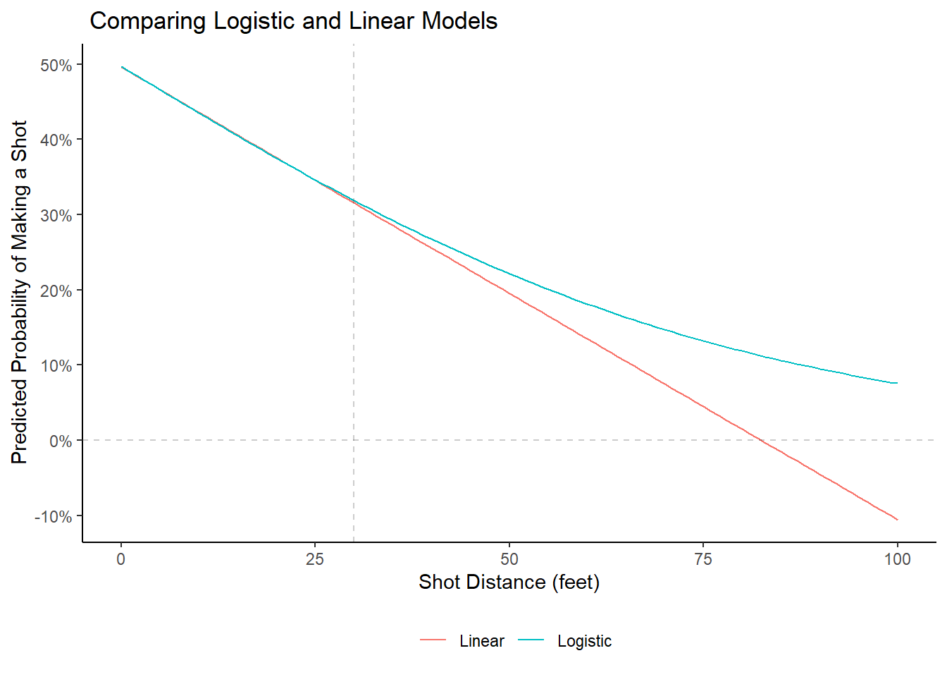
Of course, our shot data is limited to shots within about 30 feet of the rim. The plot was extended (up to 100 feet) to emphasize the difference between the two models. Both models predict essentially the same probability for making a shot for the first 30 feet. However, the linear model predicts negative probabilities for shots further than 80 feet or so. A probability can never be less than zero. This is why we go through the extra effort of working with the logistic regression.
Since the linear model is almost identical to the logistic model for the range of our data (0-30 feet), we can look at \(\beta_1\) for the linear regression model to see how an extra foot of distance affects the probability of making a shot. We have \(\beta_1 = -0.0060169\) . Player's are expected to lose approximately half a percent in their probability of making a shot for every extra foot of distance. Stated another way, the shooting percentage drops about 6% for every extra ten feet of distance. This makes sense since the predicted probability of making a shot at distance zero is roughly 0.5 and 0.32 at the 30 feet mark. This is a drop in predicted probability of 18% in 30 feet.
3.2.3 Angle Logistic Regression Model
## # A tibble: 2 x 5
##   term           estimate std.error statistic   p.value
##   <chr>             <dbl>     <dbl>     <dbl>     <dbl>
## 1 (Intercept)    -0.529     0.122       -4.32 0.0000156
## 2 abs(theta_deg)  0.00332   0.00197      1.69 0.0914
As expected from our exploratory plots, we see that the p-value for the angle coefficient is not significant at 5%. There was no clear relationship between the absolute value of the angle and the accuracy of the shooters. It wasn't like there was an obvious decrease or increase in accuracy as the players moved away from the center line.
The small but positive nature of the angle coefficient suggests that the log odds of making a shot slightly increase as you move away from the center holding the distance and player constant. In other words, the model predicts a slight increase in shooting percentage when rotating away from the center line. This result could be tested experimentally but we can doubt this prediction given the magnitude and significance of the coefficient. Intuitively, we would expect the accuracy of players to be highest from the center. Furthermore, there might be left-right difference which weren't picked up by the model since we took the absolute value of the angle. More data is needed to make further inference.
3.2.4 Player Logistic Regression Model
We can also try to quantify the effect of who is shooting the ball on the probability of making a shot. Naturally, we can expect the shooter to have a significant impact on whether the shot is likely to go in or not. Afterall, the field goal percentages of the shooters varied greatly (refer to lollipop chart above).
## # A tibble: 18 x 5
##    term            estimate std.error statistic p.value
##    <chr>              <dbl>     <dbl>     <dbl>   <dbl>
##  1 (Intercept)      -0.223      0.387   -0.576   0.565
##  2 playerPlayer 2   -1.10       0.683   -1.61    0.108
##  3 playerPlayer 3   -0.606      0.458   -1.32    0.186
##  4 playerPlayer 4    0.455      0.477    0.953   0.341
##  5 playerPlayer 5    0.0953     0.485    0.196   0.844
##  6 playerPlayer 6   -0.788      0.701   -1.13    0.260
##  7 playerPlayer 7   -0.188      0.422   -0.445   0.656
##  8 playerPlayer 8   -0.971      0.529   -1.83    0.0667
##  9 playerPlayer 9   -0.182      0.599   -0.305   0.761
## 10 playerPlayer 10  -0.273      0.455   -0.600   0.548
## 11 playerPlayer 11  -0.265      0.424   -0.625   0.532
## 12 playerPlayer 12  -0.470      0.535   -0.878   0.380
## 13 playerPlayer 13   0.0408     0.416    0.0982  0.922
## 14 playerPlayer 14   0.0783     0.417    0.188   0.851
## 15 playerPlayer 15  -0.0645     0.587   -0.110   0.912
## 16 playerPlayer 16   0.580      0.627    0.925   0.355
## 17 playerPlayer 17   0.629      0.468    1.34    0.180
## 18 playerPlayer 18  -1.39       0.671   -2.07    0.0388
Notice how the intercept coefficient is set to Player 1 by default. As a result, all players are compared to Player 1. This just happens to be relevant since Player 1's field goal percentage is 44.44% which is close to the team average of 41.36%. In other words, the model is comparing each player's shooting percentage to roughly the team average. The only statistically significant coefficient is for Player 18. This is not surprising considering the dismal 16.67 shooting percentage of Player 18.
We can fit a logistic model with no intercept to get the log odds of each player to make a shot. Once that's done, we can easily convert the log odds into odds and probabilities.
## # A tibble: 18 x 4
##    player    log_odds  odds make_prob
##    <chr>        <dbl> <dbl>     <dbl>
##  1 Player 1    -0.223 0.800     0.444
##  2 Player 2    -1.32  0.267     0.211
##  3 Player 3    -0.829 0.436     0.304
##  4 Player 4     0.232 1.26      0.558
##  5 Player 5    -0.128 0.88      0.468
##  6 Player 6    -1.01  0.364     0.267
##  7 Player 7    -0.411 0.663     0.399
##  8 Player 8    -1.19  0.303     0.233
##  9 Player 9    -0.405 0.667     0.4
## 10 Player 10   -0.496 0.609     0.378
## 11 Player 11   -0.488 0.614     0.380
## 12 Player 12   -0.693 0.500     0.333
## 13 Player 13   -0.182 0.833     0.455
## 14 Player 14   -0.145 0.865     0.464
## 15 Player 15   -0.288 0.75      0.429
## 16 Player 16    0.357 1.43      0.588
## 17 Player 17    0.405 1.50      0.6
## 18 Player 18   -1.61  0.200     0.167
Note that the predicted make_prob column is identical to the field goal percentage of each player. The model is essentially using field goal percentages to predict whether a shot will go in or not. Of course, the technique is not ideal since not all shots are created equal. Maybe the player with low shooting percentages have been taking some tough three pointers and vice versa. Using strictly their field goal percentage to predict their probability of making a layup is obviously a flawed approach.
3.2.5 The Full Model
Let's try to create a full model to try to predict the probability of making a shot given the shot distance, the angle relative to the center of the court, and the player who's taking the shot.
##
## Call:
## glm(formula = shot_made_numeric ~ dist_feet + theta_deg + player +
##     0, family = "binomial", data = shots)
##
## Deviance Residuals:
##     Min       1Q   Median       3Q      Max
## -1.4320  -1.0430  -0.8056   1.2616   1.9945
##
## Coefficients:
##                  Estimate Std. Error z value Pr(>|z|)
## dist_feet       -0.024717   0.007742  -3.193  0.00141 **
## theta_deg        0.001784   0.001021   1.748  0.08051 .
## playerPlayer 1  -0.112976   0.390403  -0.289  0.77229
## playerPlayer 2  -1.198489   0.567170  -2.113  0.03459 *
## playerPlayer 3  -0.608828   0.256300  -2.375  0.01753 *
## playerPlayer 4   0.384707   0.283601   1.357  0.17494
## playerPlayer 5   0.225292   0.310151   0.726  0.46760
## playerPlayer 6  -0.598452   0.596688  -1.003  0.31588
## playerPlayer 7  -0.030622   0.204563  -0.150  0.88101
## playerPlayer 8  -0.600019   0.400173  -1.499  0.13377
## playerPlayer 9  -0.197254   0.461457  -0.427  0.66905
## playerPlayer 10 -0.306944   0.249914  -1.228  0.21937
## playerPlayer 11 -0.075098   0.212681  -0.353  0.72401
## playerPlayer 12 -0.357033   0.385394  -0.926  0.35423
## playerPlayer 13  0.226527   0.203341   1.114  0.26527
## playerPlayer 14  0.292551   0.206556   1.416  0.15668
## playerPlayer 15  0.319131   0.474453   0.673  0.50118
## playerPlayer 16  0.412564   0.496118   0.832  0.40564
## playerPlayer 17  0.491539   0.266352   1.845  0.06497 .
## playerPlayer 18 -1.124337   0.566803  -1.984  0.04730 *
## ---
## Signif. codes:  0 '***' 0.001 '**' 0.01 '*' 0.05 '.' 0.1 ' ' 1
##
## (Dispersion parameter for binomial family taken to be 1)
##
##     Null deviance: 1612.3  on 1163  degrees of freedom
## Residual deviance: 1520.9  on 1143  degrees of freedom
## AIC: 1560.9
##
## Number of Fisher Scoring iterations: 4
Let's try to interpret some of these coefficients. As expected, the distance coefficient is significant and the log odds of making a shot decrease by 0.0247172 for every additional foot away from the basket. This effect is almost identical to the effect observed earlier for the distance-only logistic regression model.
The same is true for the angle coefficient. It very similar to the coefficent of the angle-only model. It is not significant at 5% but is significant at 10%.
Now let's look at the estimates for the players. We see that some players have negative coefficients (decrease in log odds of making a shot) while others have positive coefficients. We can sort the players by their predicted probability of making a shot to get a better understanding of their coefficients.
## # A tibble: 18 x 8
##    player    log_odds  odds make_prob real_fg   diff p_value significant
##    <chr>        <dbl> <dbl>     <dbl>   <dbl>  <dbl>   <dbl> <lgl>
##  1 Player 17   0.492  1.63      0.620   0.6   0.0205  0.0650 FALSE
##  2 Player 16   0.413  1.51      0.602   0.588 0.0135  0.406  FALSE
##  3 Player 4    0.385  1.47      0.595   0.558 0.0373  0.175  FALSE
##  4 Player 15   0.319  1.38      0.579   0.429 0.151   0.501  FALSE
##  5 Player 14   0.293  1.34      0.573   0.464 0.109   0.157  FALSE
##  6 Player 13   0.227  1.25      0.556   0.455 0.102   0.265  FALSE
##  7 Player 5    0.225  1.25      0.556   0.468 0.0880  0.468  FALSE
##  8 Player 7   -0.0306 0.970     0.492   0.399 0.0937  0.881  FALSE
##  9 Player 11  -0.0751 0.928     0.481   0.380 0.101   0.724  FALSE
## 10 Player 1   -0.113  0.893     0.472   0.444 0.0273  0.772  FALSE
## 11 Player 9   -0.197  0.821     0.451   0.4   0.0508  0.669  FALSE
## 12 Player 10  -0.307  0.736     0.424   0.378 0.0455  0.219  FALSE
## 13 Player 12  -0.357  0.700     0.412   0.333 0.0783  0.354  FALSE
## 14 Player 6   -0.598  0.550     0.355   0.267 0.0880  0.316  FALSE
## 15 Player 8   -0.600  0.549     0.354   0.233 0.122   0.134  FALSE
## 16 Player 3   -0.609  0.544     0.352   0.304 0.0485  0.0175 TRUE
## 17 Player 18  -1.12   0.325     0.245   0.167 0.0785  0.0473 TRUE
## 18 Player 2   -1.20   0.302     0.232   0.211 0.0212  0.0346 TRUE
We see that players with a predicted probability of a made shot above 50% have positive coefficients. Another interesting thing to note is that the predicted probability of making a shot for a specific player is not the same as their overall field goal percentage. This was the case for the angle-only logistic regression model. In fact the predicted probabilities are consistently higher than the actual field goal percentages. This makes sense since the full model is trying to isolate the player's shooting ability independent of the location of their shots while the play-only model only considered the name of the player and not where they were shooting from.
The only players with significant coefficients are Player 3, Player 18, and Player 2. This implies that these players are shooting worse than the others independent of where they're shooting from. Player 17's coefficient is almost significant at 5% which gives us some evidence that they are shooting better than others independent of shot location.Some honorable mentions in terms of significance could go to Player 4 (good), Player 14(good), and Player 8 (bad).
## # A tibble: 2 x 5
##   player    make_prob real_fg   diff p_value
##   <chr>         <dbl>   <dbl>  <dbl>   <dbl>
## 1 Player 18     0.245   0.167 0.0785  0.0473
## 2 Player 2      0.232   0.211 0.0212  0.0346
Furthermore, it is worth noting that the model predicted Player 2 to be a worse shooter than Player 18 although Player 2 had a higher field goal percentage. The reason for this becomes evident once we compare their shot charts.
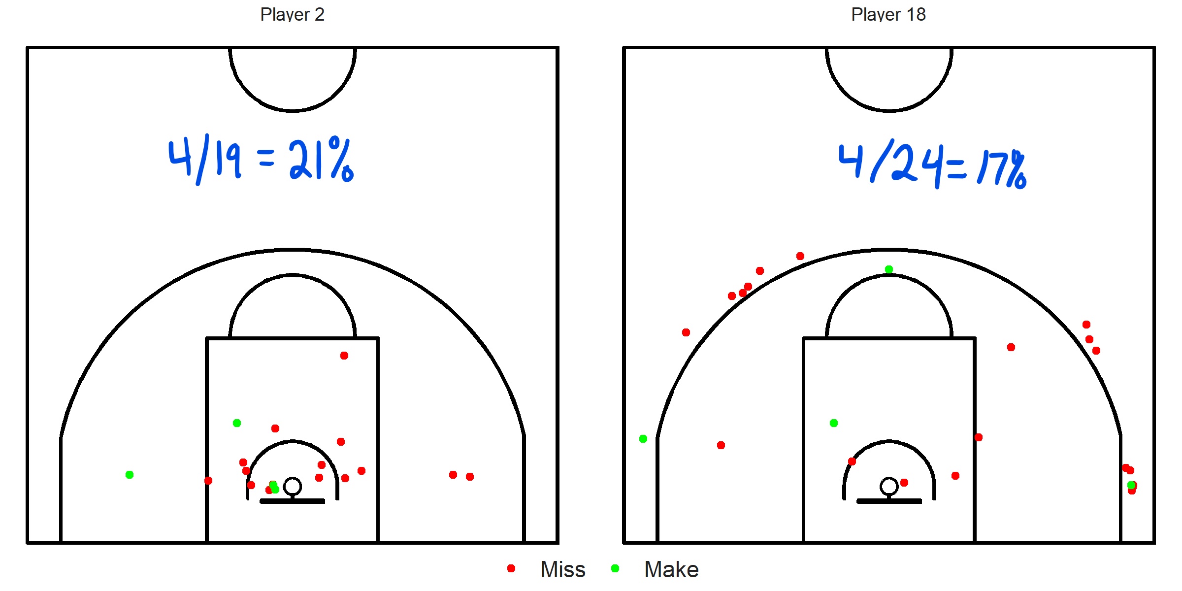
Player 18 is taking harder shots than Player 2. Therefore, when controlling for distance and angle, the model predicts that Player 18 is better shooter despite the lower field goal percentage.
## # A tibble: 10 x 6
##    player    dist_feet theta_deg make_prob_dist make_prob_full outcome
##    <fct>         <dbl>     <dbl>          <dbl>          <dbl>   <dbl>
##  1 Player 10     22.9     49.0            0.358          0.313       0
##  2 Player 13      1.56    97.6            0.487          0.590       1
##  3 Player 14     24.8     -0.822          0.347          0.420       1
##  4 Player 17      1.74  -102.             0.486          0.566       0
##  5 Player 5       3.99   -80.3            0.472          0.496       0
##  6 Player 13     24.1    -48.0            0.352          0.388       0
##  7 Player 11      7.78   -37.3            0.449          0.417       0
##  8 Player 8      22.9     86.7            0.358          0.267       0
##  9 Player 3       5.18   -15.6            0.465          0.318       0
## 10 Player 2      16.5    -87.0            0.395          0.146       0
Lastly, the table above compares the predictions of the distance-only model to the predictions of the full model. We can see that the full model has some predictions which are over 50% which isn't the case for the distance model. We can see in row 2 and 4 that the distance model assigns a probability of 48% to both player of making the lay up while the full model gives the edge to Player 13 over Player 17.
3.3 Closing Thoughts
We barely scratched the surface of what is possible to do when modeling basketball shots. The aim of this chapter was twofold. First, it was meant to serve as an introduction to the key ideas and techniques of statistical modeling. Second, this chapter was designed to build some intuition about what constitutes a "good" shot attempt in basketball. This intuition will be vital to carry out the spatial analysis in the coming chapters.
The next chapter will explore how we can use the predicted probabilities from our logistic regression models to try to predict whether shots will go in or not.
Note that all the R code used in this book is accessible on GitHub.