4 Classification of Basketball Shots

Note that all the R code used in this book is accessible on GitHub.

A sensible thing to do with basketball shot data is to try to guess³³ which shots are going to go in.

4.1 No Information

Let's say we know nothing about a basketball shot. We don't know who is shooting and from where, nor do we know the overall field goal percentage. The only thing we can do with zero information is to give an equal chance to both outcomes. In Bayesian statistics, this is the simplest non-informative prior or often reffered to as the Principle of Indifference. Note that frequentists don't think it makes sense to ask about the probability of a single event occurring without thinking of the long-term relative frequencies³⁴.

Nevertheless, let's see how accurate it is to randomly classify half of the shots as makes and the other half as misses. This will serve as our baseline to see if we can improve on this accuracy by adding more information.

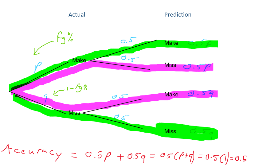
Figure 4.1: Flipping a coin to see which shots are going in

We can create a tree diagram like the one above to theoretically figure out that we can expect to classify somewhere around 50% of the shots correctly if we were to guess at random. We can also verify this result experimentally with a simulation.

# Number of replications
B <- 500

# Create an empty vector to store the accuracies of each replication
accuracies <- vector(length = B)

# Create a vector for whether the shots actually went it
actual_response <- shots$shot_made_numeric

# Set the seed to ensure reproducibility
set.seed(2021)

# Perform Simulation
for(i in 1:B){
  # Randomly generate 1s and 0s based on equal 50-50 probabilities
  predicted_response <- sample(
  x = c(0, 1), size = nrow(shots), replace = TRUE,
  prob = c(
    0.5, # Miss probability
    0.5) # Make probability
  )
  
  accuracies[i] <- (table(predicted_response, actual_response)[1, 1] +
     table(predicted_response, actual_response)[2, 2]) /
    length(actual_response)
}

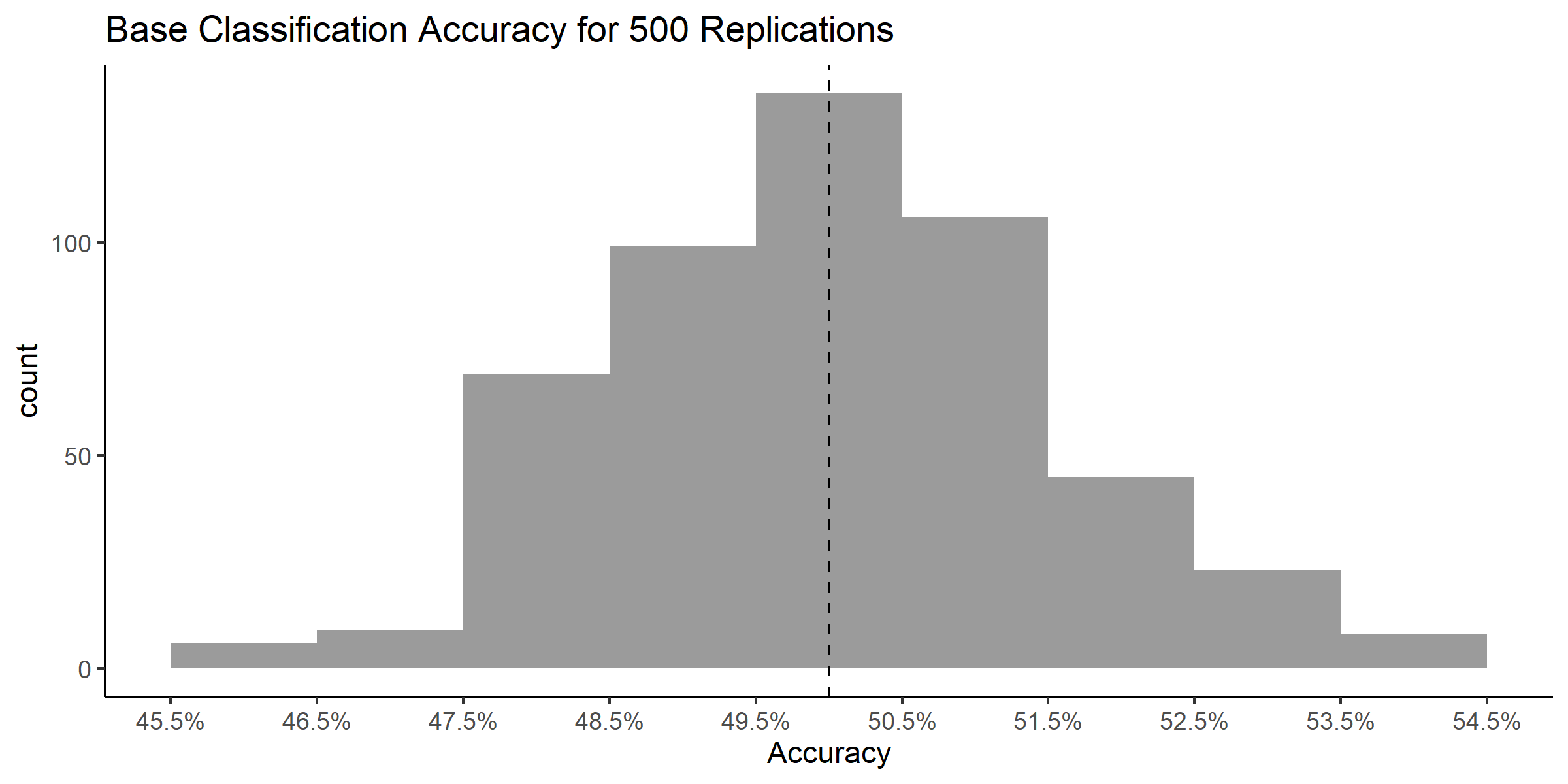
Figure 4.2: The simulation accuracy hovered around 50%

We essentially flipped a coin to decide whether each of the 1163 shots were going to go in or not and kept track of how many times we were right³⁵. Then, we repeated this process 500 times. We see that the empirical accuracy did indeed hover around the theoretical accuracy of 50%.

4.2 Overall Field Goal Percentage

If we knew the overall field goal percentage of the sample, then we could use a slightly more informed approach. We could flip a weighted coin that had a 41.36% chance of landing heads (make) and a 58.64% chance of landing tails (miss), then we can expect to predict about 51.49% of the shots correctly. This result can be verified experimentally by running a simulation and theoretically by building a tree diagram like the one below.

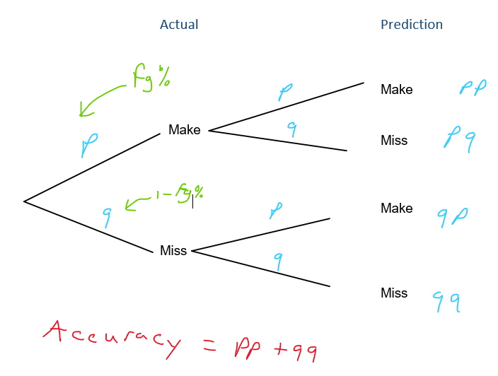
Figure 4.3: Using a weighted coin to predict shot outcomes

This means that knowing the overall field goal percentage in the sample helps us predict the outcome of the shot about an extra 1.49% of the time (51.49 - 50). This is a slight improvement. However, knowing the individual player's shooting percentages may be more predictive.

4.3 Shooter

Since we already calculated the field goal percentages of each player in Chapter 3, it's simple to predict whether the shot will go in or not. A common approach is to say that the shot will go in if the predicted probability is greater than 50%.

\[P(X) = P(Y = \mbox{Make} ~| ~ X = \mbox{shooter})> 0.5\]

This should make sense intuitively. If you had to bet on whether a given shot goes in or not, the first thing you would try to figure out is whether the player is more likely to make it or not. We can naively adopt this approach.

The results of our classification can be summarized in a confusion matrix like the one below.

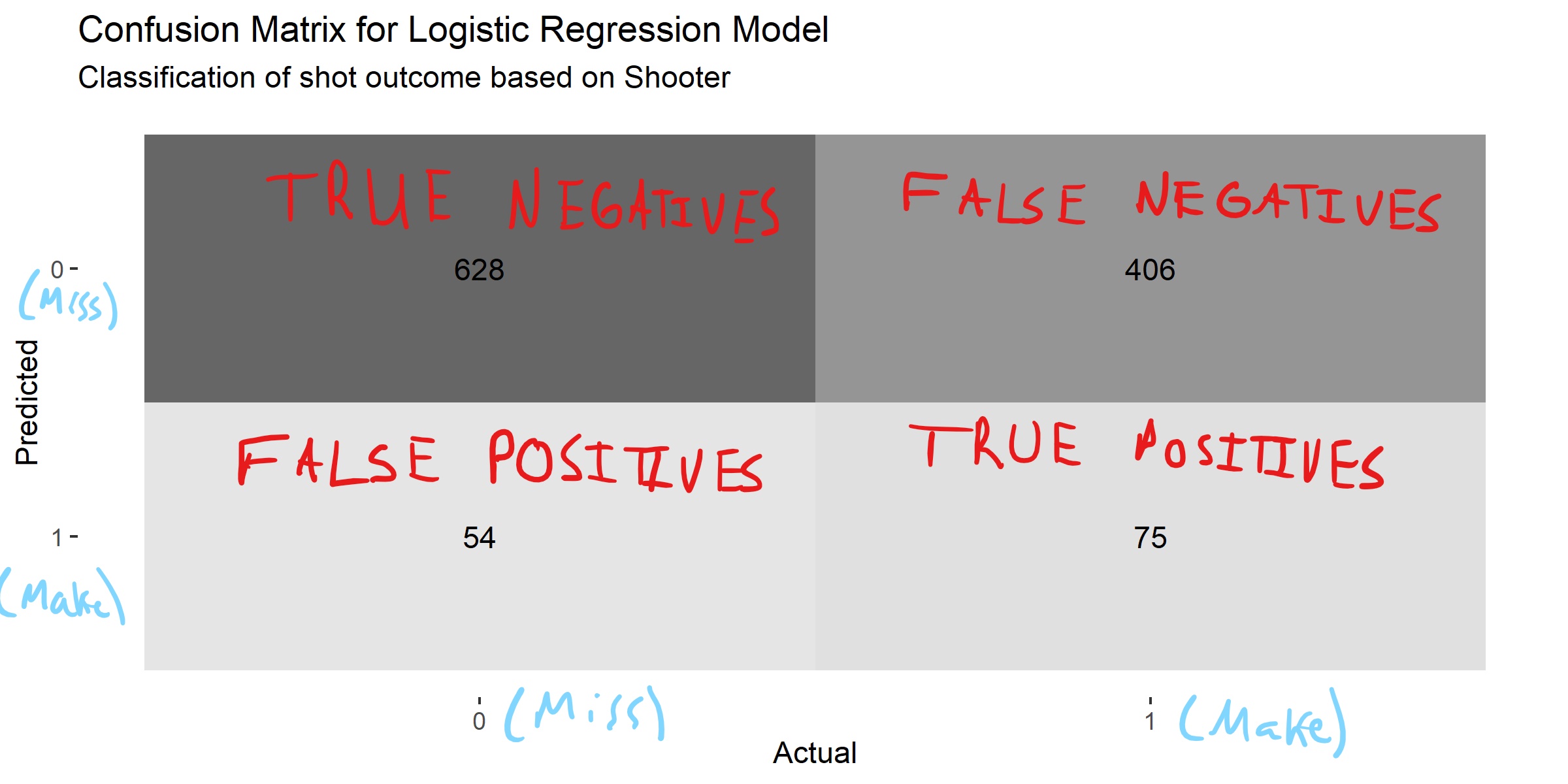
Figure 4.4: Deconfusing the confusion matrix

Table 4.1: Summary statistics for player-only classification attempt

.metric	.estimate
accuracy	0.604
sens	0.156
spec	0.921

We see that simply knowing who shot the ball can improve our accuracy to 60.45%. This is a significant improvement from 50% and 51.49%.

However, this improved accuracy needs to be contrasted with the fact that predicting that every shot will miss gives us an accuracy of 58.64%.

Thus, our model does only slightly better than predicting all misses. It correctly predicts makes only 15.59% of the time and correctly predicts misses 92.08% of the time³⁶. A rule of thumb is that we want both the sensitivity and specificity to be above 80%.

We can look under the hood to see why this is happening. Only three players make over 50% of their attempts³⁷. As a result, the model predicts that all of their shots are going to go in and everyone else's shots are going to miss. This explains why there are only 75 true positives and 406 false negatives.

We could try to lower the positive prediction threshold to increase the number of predicted makes. Let's say that everyone who shoots better than the team average (41.36%) will be predicted to make their shots and everyone who shoots worse than the average will miss.

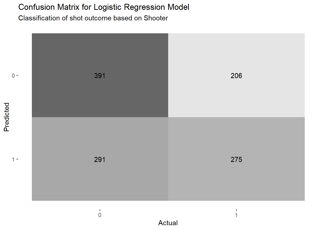
Figure 4.5: Lowering the bar from 50% to the the team average of 41.36%

Table 4.2: Player-only classification attempt with lower threshold

.metric	.estimate
accuracy	0.573
sens	0.572
spec	0.573

We see that the accuracy of the model dropped slightly. Furthermore, the sensitivity increased significantly at the expense of the specificity. Only knowing who shot the ball is better than nothing but there's a ton of room for improvement.

4.4 Shot Angle

Let's try to see how effective knowing the angle from the center line is at classifying shots in our sample.

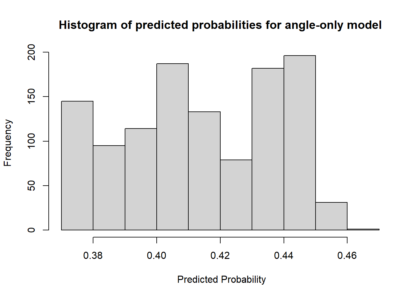
Figure 4.6: All predicted probabilities are below 50%

The classification accuracy of the angle-only model is 58.64%. This seems decent at first glance but the confusion matrix reveals that it predicted that all shots were going to miss. We saw in the previous chapter that there was no clear relationship between the angle from the center and the probability of making the shot. Thus, we won't investigate this model further.

4.5 Shot Distance

Using the distance-only model will initially give the same result as the angle-only model. This is easy to see since even a shot at the rim (distance = 0) results in a probability of less than 50%.

\[ P(Y = \mbox{Make} ~| ~ X = 0)= \frac{e^{\beta_0 + \beta_1 (0)}}{e^{\beta_0 + \beta_1(0)} + 1} = \frac{e^{\beta_0}}{e^{\beta_0} + 1} = \frac{e^{-0.0124199}}{e^{-0.0124199} + 1} \approx 0.497 \] We saw that the predicted probabilities dropped roughly linearly for the range of our sample³⁸. We can inspect the distribution of predictions to decide on a better threshold than 50%.

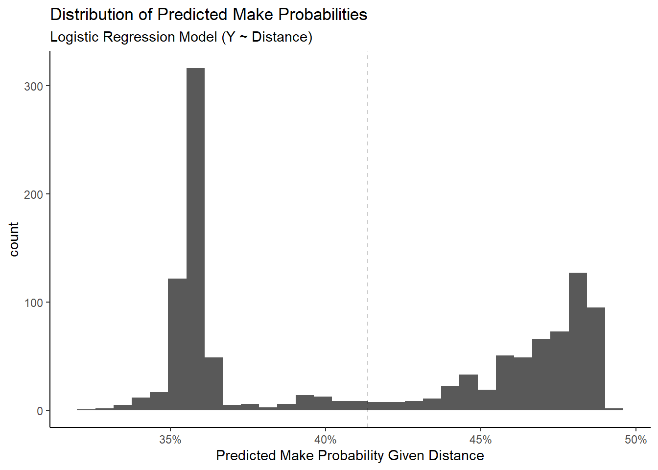
Figure 4.7: All predicted probabilities are also below 50%

We see that the model never predicts that the shot is going to go in if \(P(X)\) needs to be greater than 50%. The overall shooting percentage in the sample is 41.36%. Thus, if we knew nothing about the location of the shot, it would make sense to bet on the player not making the shot based on the overall shooting percentage being less than 50%.

Most predicted make probabilities are between 35% and 50% and there seems to be a bimodal distribution of probabilities. This is almost certainly explained by the fact that the shot distances also had a bimodal distribution with most shots near the rim and at the three-point line ³⁹.

We can try to classify shots with a threshold of 41.36% instead of 50%. This would roughly be the same as predicting that all shots further than 14 feet away are going to miss while any attempt closer than this distance will make it.

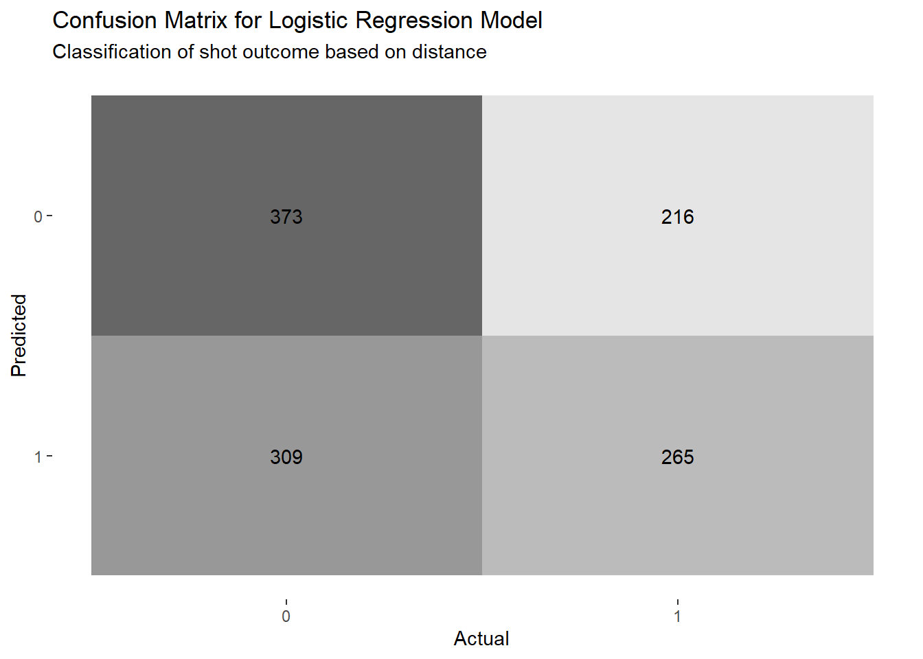
Figure 4.8: Lowering the bar from 50% to the the team average of 41.36%

Table 4.3: Distance-only classification attempt with lower threshold

.metric	.estimate
accuracy	0.549
sens	0.551
spec	0.547

Of course, this classification approach is very limited. Our distance logistic regression model was able to correctly predict the outcome of 58.64% of the shots in our sample. Is this impressive? It is better than flipping a coin but worse than predicting that all shots were going to miss.

4.6 Knowing All Three

Finally, let's use all the information we have available to try to accurately classify shots as makes or misses. We will use the full logistic model with distance, angle, and player⁴⁰.

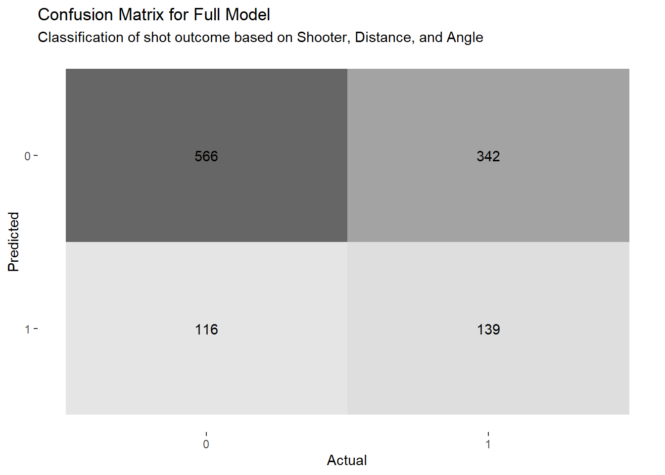
Figure 4.9: Classification results for the full model

Table 4.4: Full model classification metrics

.metric	.estimate
accuracy	0.606
sens	0.289
spec	0.830

We see that the full model has a classification accuracy of 60.62%. We could try to improve this by lowering or increasing the 50% threshold but the default value seems reasonable based on Figure 4.10 below.

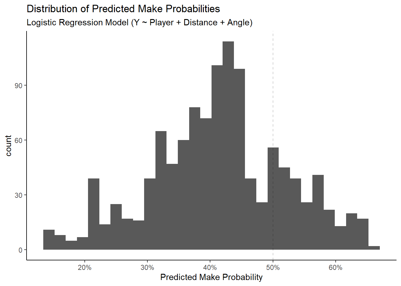
Figure 4.10: A significant proportion of shots have a predicted probability above 50%

4.7 Closing Thoughts

We saw that we could correctly predict the outcome of a basketball shot about 50% of the time if we flipped a fair coin. Knowing the overall field goal percentage of the sample allowed us to make slightly better predictions with an accuracy of 51.49%. We would have been correct 58.64% of the time if we predicted that all shots were going to miss. Knowing who shot the ball had an accuracy of 60.45%. Only knowing the shot distance resulted in an accuracy of 58.64% (predicted all misses). The same was true about only considering the shot angle. Lastly, using all the information available resulted in a classification accuracy of 60.62%. We can summarize the results in Table 4.5 below.

Table 4.5: Comparing the different classification approaches

Available Information	Accuracy
None	50.00%
Overall FG%	51.49%
Individual FG%	60.45%
Shot Angle	58.64%
Shot Distance	58.64%
All	60.62%

Knowing the individual players' field goal percentages was the most potent information when it came to predicting the outcome of each shot in our sample. The long-term shooting percentages are almost never known in advance which is where the other information such as the distance from the hoop distance and the angle from the center can come in handy. A slight increase in classification accuracy may not have a drastic impact in terms of playing strategy, but it can have immediate applications to sports gambling for example or long term predictions.

One can imagine that adding other variables such as the distance from the shooter to the closest defender, the player's speed prior to the shot, whether the shot was off the dribble or not, and the time on the shot clock could help incrementally raise the accuracy of our predictions. Having access to the initial conditions of each shot could one day classify shots in a near deterministic fashion.

Now that we've got acquainted with our data and a general modeling framework, let's try to build a FIBA basketball court in R using the sf package.

Note that all the R code used in this book is accessible on GitHub.