8 Point Pattern Analysis

Note that all the R code used in this book is accessible on GitHub.

Now that we've built spatial objects for the basketball shots and basketball court, we can finally start investigating the spatial structure of the data. Point pattern analysis is the typical name for this sort of investigation. The focus of this chapter is to explore the spatial distribution of the shot locations.

Let's load the spatial shots, the basketball court, and the spatial polygons we've built in the previous chapters. Additionally, we can load the spatstat package for its point pattern analysis functions.

# Load libraries
library(spatstat)
library(tidyverse)
library(sf)

# Load the plot_court() function from the previous chapters
source("code/court_themes.R")
source("code/fiba_court_points.R")
# Load the different zone polygon objects
source("code/zone_polygons.R")

# Load shot spatial data
shots_sf <- readRDS(file = "data/shots_sf.rds")

The analysis below was heavily influenced by Adam Dennett's publicly accessible tutorials. Let's plot our data so we have an idea of what we are working with.

plot_court() +
  geom_sf(data = shots_sf, aes(color = shot_made_factor),
          alpha = 0.1, size = 1) +
  # Red = Miss, Green = Make
  scale_color_manual(values = c("red", "green")) +
  # Remove legend title
  theme(legend.title = element_blank())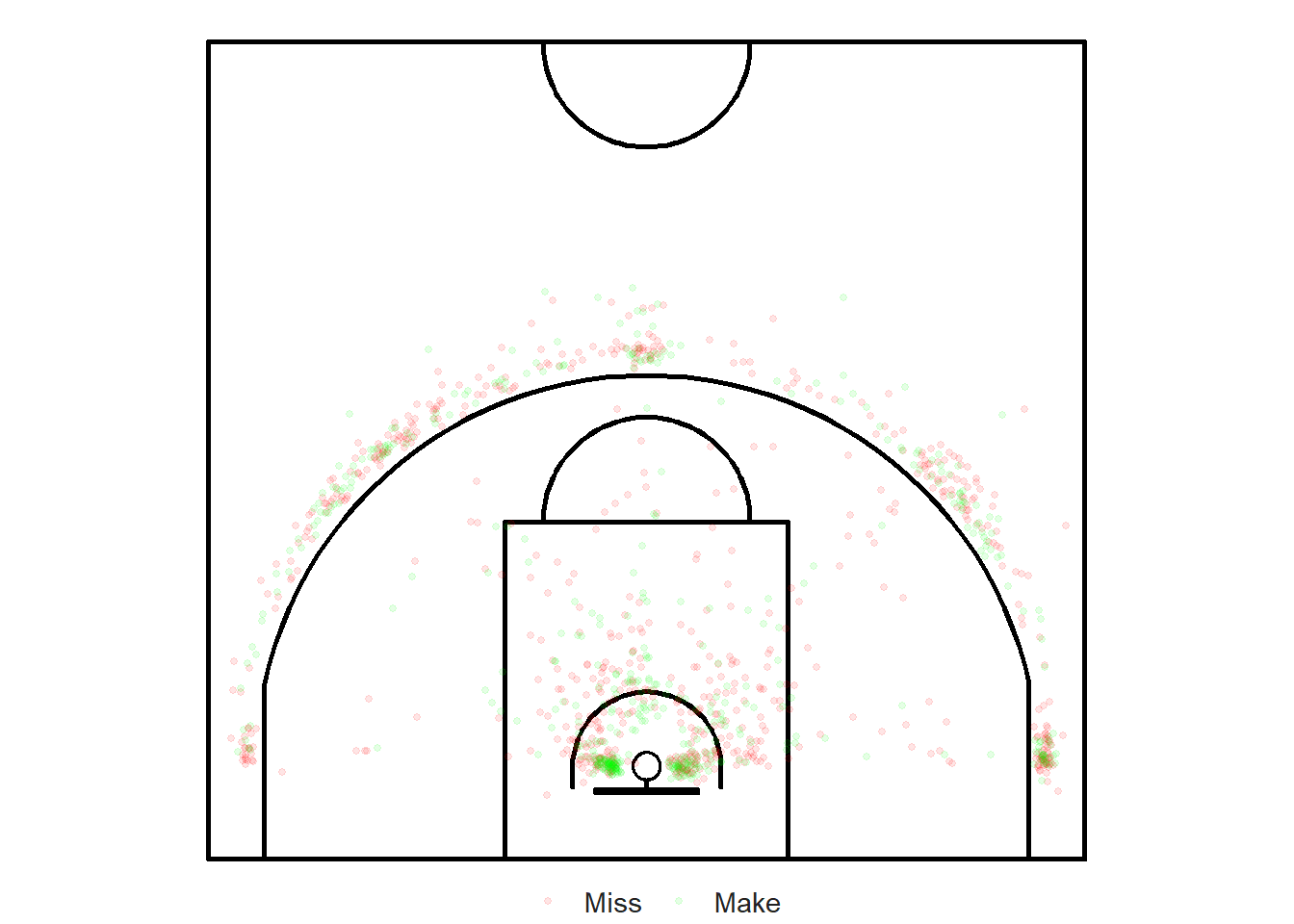

Figure 8.1: The eye-test seems to indicate the presence of clustering

8.1 Quadrat Analysis

The question we want to answer is:

Are the shots distributed randomly⁴⁶ or do they exhibit some kind of dispersed or clustered pattern?

Another way of saying this is:

Does the distribution of shot locations differ from complete spatial randomness (CSR)⁴⁷?

8.1.1 Hypotheses

We can formalize this by proposing the following hypotheses:

\[ \begin{aligned} H_0 &: ~~\mbox{shot locations are completely spatially random} \\ H_A &: ~~\mbox{shot locations are NOT completely spatially random} \end{aligned} \]

The easiest way to test this hypothesis is to conduct a quadrat test. To do this, we need to split up the court into a grid and count the number of shots that fall within each cell of the grid. We will use the quadratcount() function from the spatstat package to achieve this.

8.1.2 Observation Window

But first, we need to create an observation window to inform the package which region of the court we are interested in. We could use the entire half-court (or the full-court for that matter), but the vast majority of the shots were taken between the backboard and a few feet past the three-point line. Therefore, we will create a window that is essentially a circle centered at the hoop with a radius of 7.75 meters. The circle is cropped to fit within the court and to be above the backboard.

# Define a point sfg object for the center of the hoop
hoop_center <- st_point(c(width/2, hoop_center_y))

# Create a circle with radius 9 and crop it to fit within the court
window_points <- st_crop(
  st_sfc(st_buffer(hoop_center, dist = 7.75)),
  xmin = 0, ymin = backboard_offset - backboard_thick,
  xmax = width, ymax = height
)

# Create a polygon sf object with the coordinates
window_points <- st_polygon(list(
  st_coordinates(window_points)[ , 1:2]
  ))

# Define a window based on where the shots tend to take place
window <- as.owin(window_points)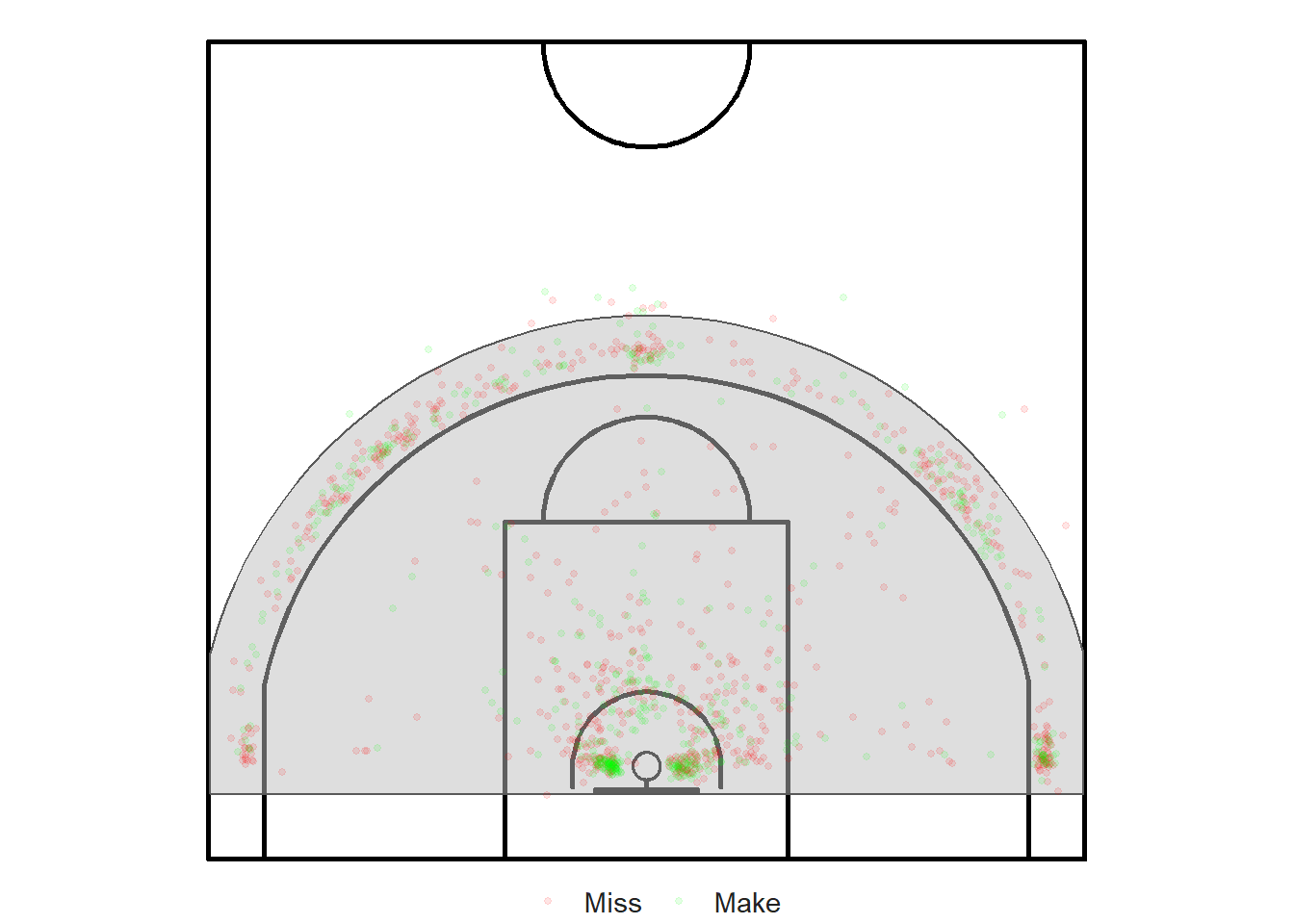

Figure 8.2: Observation window for our quadrat analysis

The vast majority of basketball shots were released within this area. This is where the action takes place.

The spatstat package unfortunately does not yet work with sf objects. As a result, we will need to create a planar point pattern (ppp) object for the shots that fall within our observational window.

# only keep the shots that are in the window
shots_window <- shots_sf[window_points, ]

# Create a ppp object
shots_ppp <- ppp(
  x = st_coordinates(shots_window)[, 1],
  y = st_coordinates(shots_window)[, 2],
  window = window)

8.1.3 Quadrat Test

Now we can use the quadratcount() function from the spatstat package and plot the results.

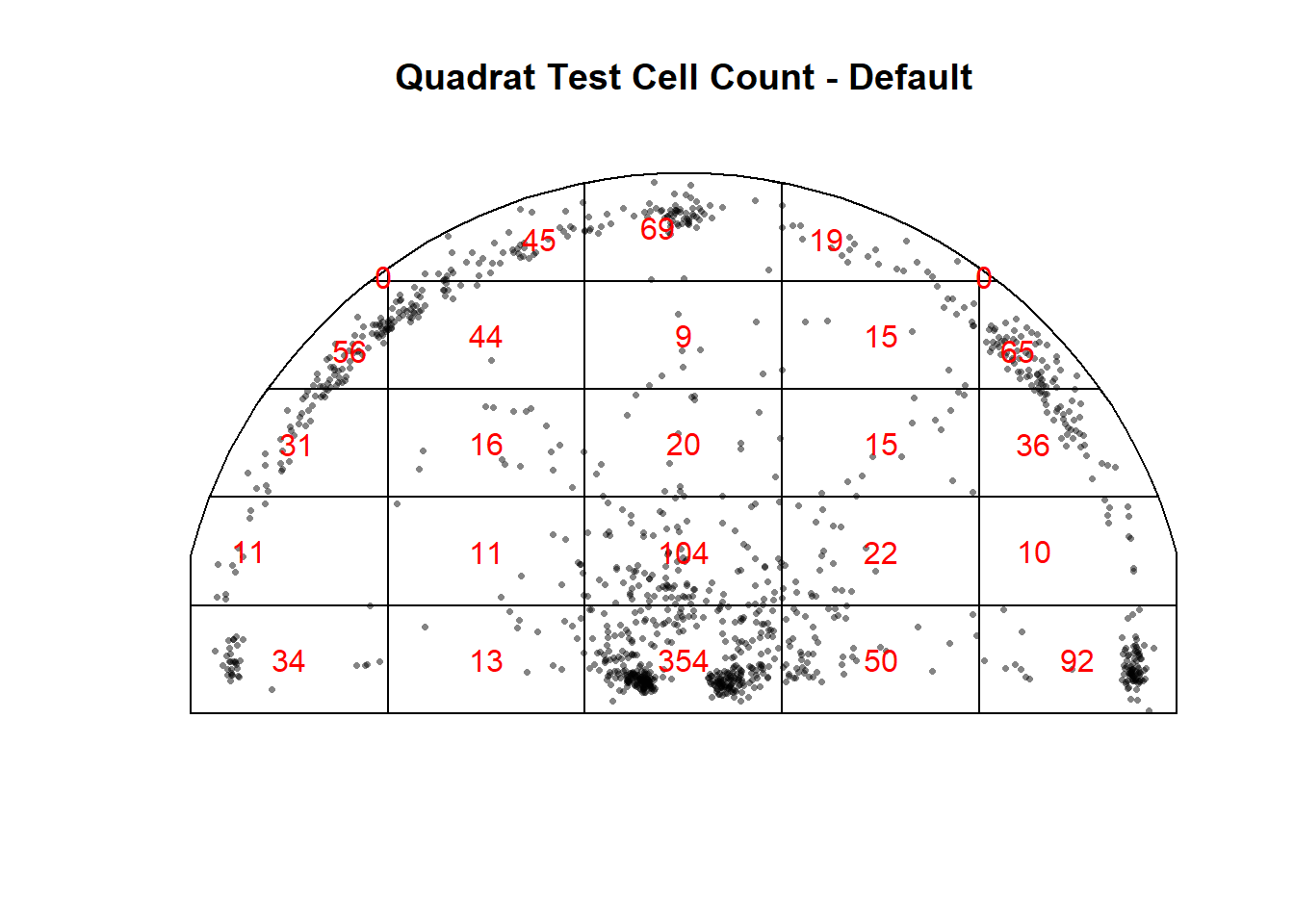
Figure 8.3: Are the cell counts random?

If the shots were spatially random, then we can imagine that the observed number of points within each cell would be similar for all equally sized cells. This is definitely NOT the case in Figure 8.3.

# Conduct Quadrat Test
qtest <- quadrat.test(shots_ppp)

# Display Results
qtest

## 
##  Chi-squared test of CSR using quadrat counts
## 
## data:  shots_ppp
## X2 = 2147.9, df = 24, p-value < 2.2e-16
## alternative hypothesis: two.sided
## 
## Quadrats: 25 tiles (irregular windows)

We see that the p-value for the quadrat test⁴⁸ is very close to zero. This implies that the probability of observing the shot locations in our sample is extremely unlikely if the null hypothesis was true⁴⁹. In fact, we didn't need to calculate a p-value to reach this conclusion. We could have used a much simpler method; the interocular traumatic test⁵⁰. This test can be used when the result is so obvious that it hits you between the eyes, hence causing "inter-ocular trauma". The cell that encloses the hoop contains 354 shots. This is an order of magnitude (10X) more than most cells.

8.1.4 Chi-squared Statistic

The Chi-squared statistic for the quadrat test is defined as follows:

\[ \chi^2 = \sum_{i=1}^{25} \frac{(O_i - E_i)^2}{E_i}, \] where \(O_i\) is the observed number of shots in each cell and \(E_i\) is the expected number of shots in each cell. The red numbers in Figure 8.3 represent the observed cell counts (\(O_i\)). We can try to calculate how many shots we should expect in each cell if they had a complete spatial random distribution (\(E_i\)). We have 1141 shots in our window. The area of the cells that are equal in size is roughly \(4.95 ~m^2\) (\(3 \times 1.65\)) while the entire area of the window is \(100.78~m^2\) . Then, each of those equally sized cells should contain roughly \(1141 \times \frac{4.95~m^2}{100.8~m^2} \approx 56\) shots.

The areas for the rectangular cells are easy to calculate. However, we will use the quadrat.test() function to calculate the area of the irregularly-shaped cells for us.

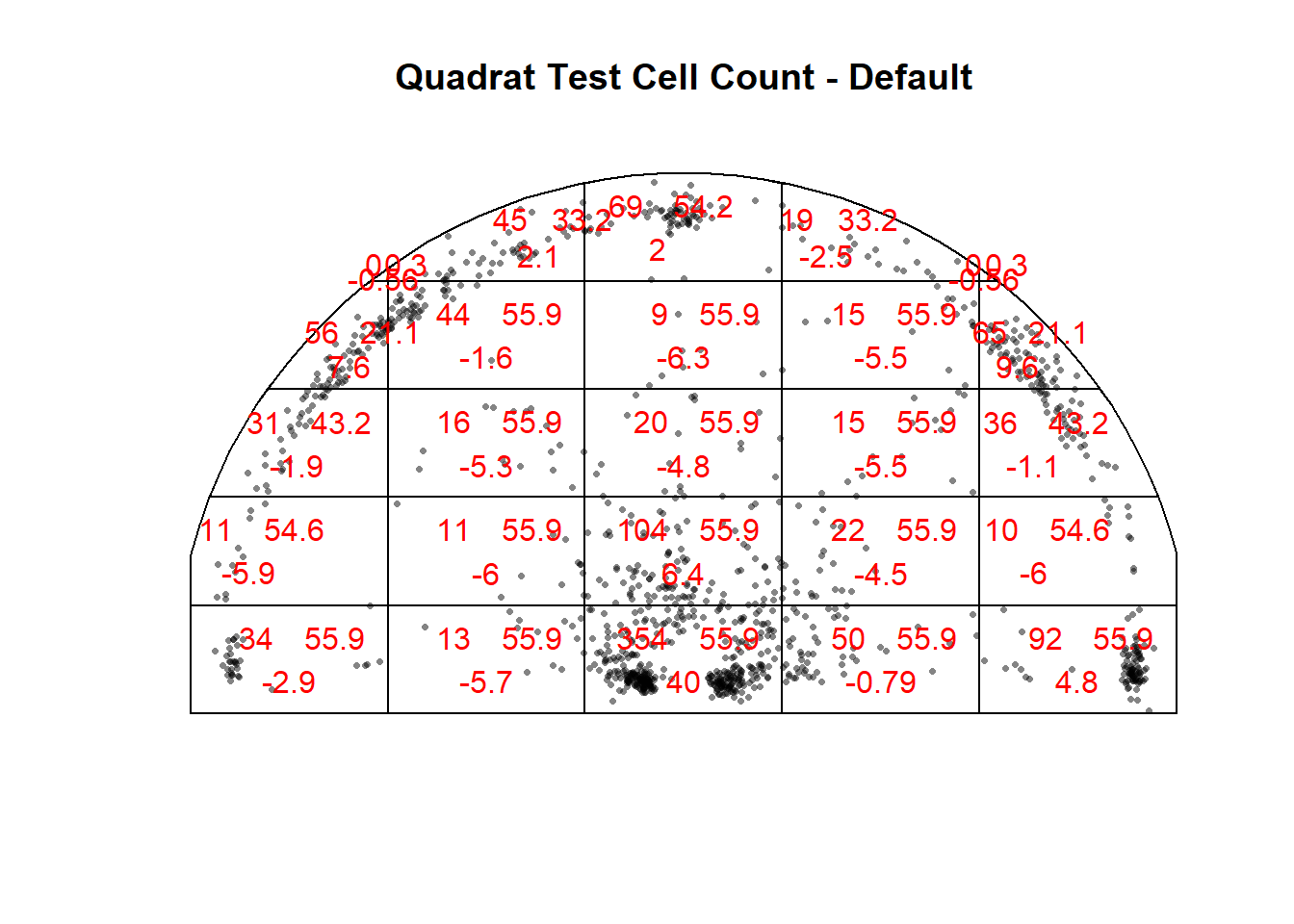
Figure 8.4: Expected shots per cell (top-right corner)

In the Figure 8.4, we can see three figures for each quadrat. The top-left number is the observed count of shots (\(O_i\)). The top-right number is the Poisson expected number of shots (\(E_i\)). Lastly, the bottom number is the Pearson residual value defined as \(\frac{O_i - E_i}{\sqrt{E_i}}\). There are three things worth pointing out about the picture above. Notice how all the rectangular cells have 55.9 in the top-right corner. This confirms the expected number of shots we calculated by-hand in the previous paragraph. Furthermore, the expected number of shots in each cell⁵¹ is proportional to the area of the cell. Lastly, the Chi-squared statistic \(\chi^2 = \sum_{i=1}^{25} \frac{(O_i - E_i)^2}{E_i}\) is the sum of the squared Pearson residuals⁵². Thus, a larger Chi-squared value is evidence that the observed cell counts were far from the expected cell counts based on a random spatial distribution.

8.1.5 Generating Artificial Shots

We can use the st_sample() function from the sf package to randomly generate shot locations.

set.seed(2021)
csr_points_sf <- st_sample(
  x = window_points,
  size = nrow(shots_window),
  type = "random",
  exact = TRUE
)

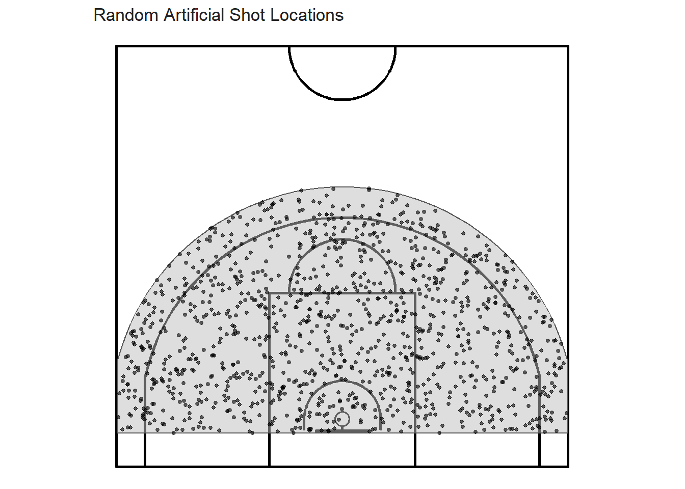
Figure 8.5: Randomly generated CSR points

The shot locations from the plot above look much more evenly distributed than the shot locations from our sample.

## 
##  Chi-squared test of CSR using quadrat counts
## 
## data:  csr_points_ppp
## X2 = 15.291, df = 24, p-value = 0.1761
## alternative hypothesis: two.sided
## 
## Quadrats: 25 tiles (irregular windows)

The p-value of the quadrat test for the artificial shots is greater than 0.05 so we can't conclude that the shot locations are not completely spatially random.

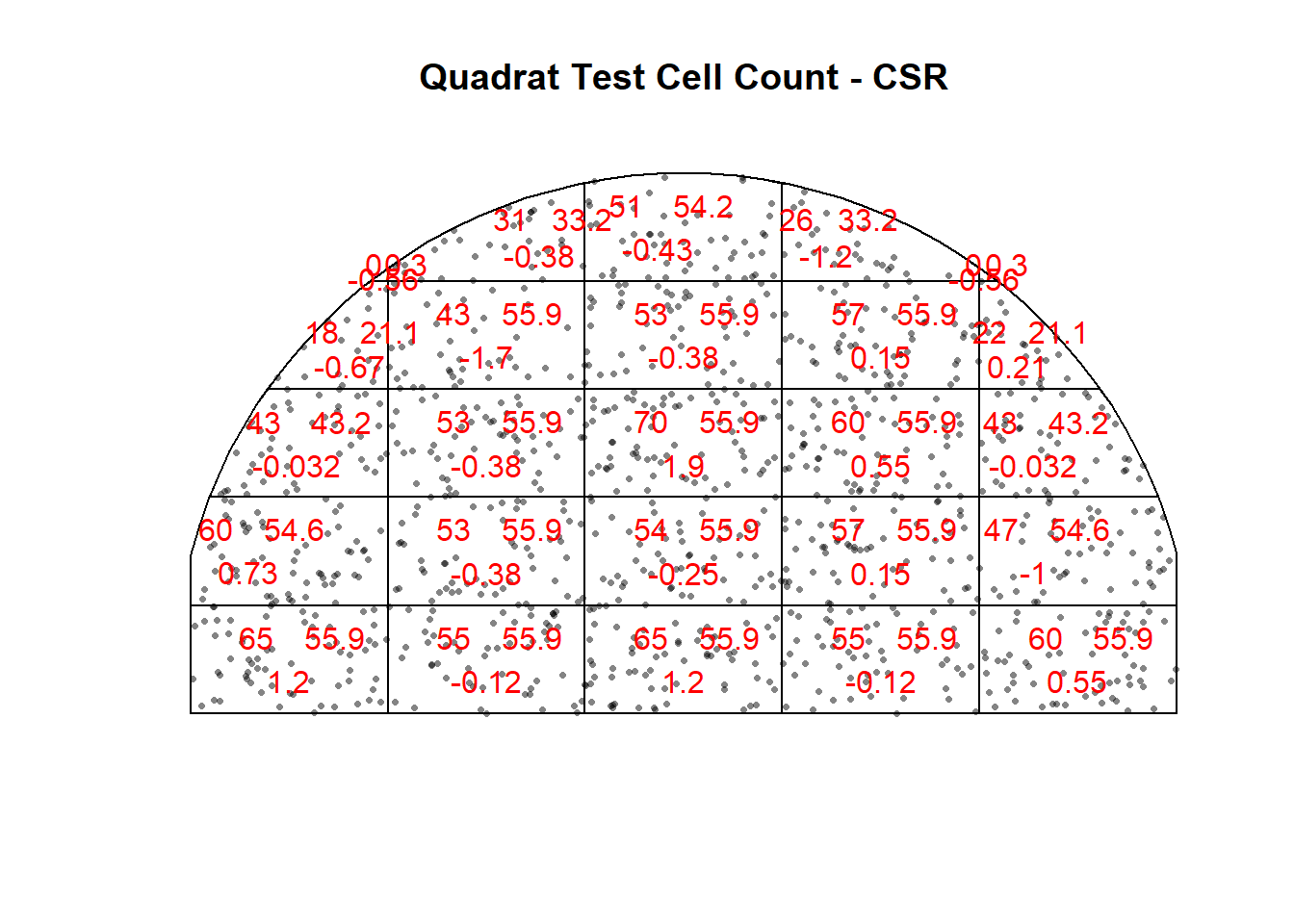
Figure 8.6: Randomly generated CSR points

It is not surprising that the number of observed artificial shot locations⁵³ within each cell is close to the expected number based on the Poisson distribution⁵⁴.

8.2 Further Investigation

It is pretty obvious that the shots in our sample are not random. There are some visible clusters. However, it is much less obvious when trying to answer the same question within a specific zone instead of the half-court. Quadrat analysis could be used to test whether mid-range shots follow CSR⁵⁵ for example.

8.3 Limitations

Quadrat analysis has serious limitations. First, the size of the grid cells affects the power of the quadrat test. If the cells are too large, then there won't be enough cell counts to compare to the poisson distribution. If the cells are too small, then we run the risk of not having enough shots within each cell. Second, the quadrat approach does not take into account the arrangement of points in relation to one another. Instead, it only considers the density of the points. Third, it results in a single measure for the entire distribution and variations within the each cell won't be considered.

The next chapter will try to address some of these limitations.

Note that all the R code used in this book is accessible on GitHub.

7 Basketball Shots as Spatial Objects

9 Nearest Neighbour Analysis