10 Spatial Clustering

Note that all the R code used in this book is accessible on GitHub.

Let's try to build on the findings from the previous chapters. We know that the shots appear to be clustered instead of being completely spatially random (CSR). A natural extension of this result is to investigate where such clusters may reside.

10.1 DBSCAN

We will use the DBSCAN⁶³ algorithm to try to classify the shots into groups based on the number of points nearby⁶⁴. This video shows a quick walk-through of how this technique works. I have also particularly enjoyed this article. The algorithm can be described at a high-level with the following steps:

Specify the two parameters of the algorithm.
- \(\varepsilon\) is the radius of the epsilon neighborhood⁶⁵.
- minPTS is the minimum number of core points (including starting point) required in the epsilon neighborhood for a cluster to be formed.
Randomly select a shot location (starting point).
Identify the shots (core points) in the \(\varepsilon\)-neighbourhood of the starting point.
A cluster is formed if there are at least \(n=\)minPTS core points in the \(\varepsilon\)-neighborhood of the starting point.
Once a cluster is formed, each core point will broadcast their own \(\varepsilon\)-neighbourhoods with the hope of adding new points to the cluster.
Once a cluster is complete, the algorithm repeats these steps starting at step 1 with a random point that is not already part of a cluster. If all unclustered points can't be added to a cluster, then these points are labeled as noise⁶⁶ and the process is done.

Playing around with this interactive visualization is a great way to build up some intuition about how the DBSCAN algorithm works.

10.1.1 Advantages of DBSCAN

The reasoning behind using DBSCAN over other clustering algorithms is fourfold. First, we don't need to specify the number of clusters in advance. This is crucial since although we might have a rough idea of where the shots are coming from, the purpose of using a clustering algorithm is to pick up patterns that may not be obvious by looking at a shot chart or a heatmap⁶⁷. Second, the two parameters of the algorithm (minPTS and \(\varepsilon\)) are intuitive enough to be carefully chosen by a domain expert⁶⁸. Third, DBSCAN can identify arbitrarily-shaped clusters. It is unlikely that the clusters around the rim and the clusters around the three-point line have the same shape. Fourth, this technique is robust to outliers and noise. This is necessary to adequately analyze basketball shots. A buzzer-beater half-court shot should not be considered in the same way as a lay up. For the reasons listed above, the DBSCAN clustering algorithm seems to be a proper tool for our analysis.

10.1.2 Parameter Selection

We can use the results from Chapter 9 to inform our parameter selection. Section 9.1 told us that 90% of the shots have a nearest neighbour that is located within 20 centimeters. Furthermore, Ripley's K Function from Section 9.2 gave us the average number of points within a certain radius of a random shot. Given the relatively large number of shots in our dataset⁶⁹ and the fact that the K function told us that there was an average of roughly 16 shots within a radius of 20 centimeters, it is reasonable to naively adopt these two values as good starting points for \(\varepsilon\) and minPTS. Larger values for minPTS will result in smaller more significant clusters. The same can be said about smaller values for \(\varepsilon\).

10.1.3 Naive Results

The analysis below was inspired by Adam Dennett's publicly accessible tutorials. Let's plot the results of the DBSCAN algorithm with \(\varepsilon = 0.2\) and minPTS\(= 16\).

# Load the DBSCAN library
library(dbscan)

# Convert the shots sf object to a dataframe with the xy-coordinates
shots_df <- data.frame(st_coordinates(shots_sf))

# Run the dbscan algorithm
db_naive <- dbscan(shots_df, eps = epsilon, MinPts = min_points)

# Create an sf object with the shots and cluster ID
clusters_sf <- st_as_sf(
  x = shots_sf %>% 
    mutate(cluster_id = db_naive$cluster) %>%
    filter(cluster_id >= 1)
  )

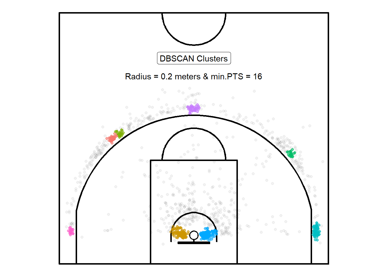
Figure 10.1: Not bad for a first attempt

Figure 10.1 displays the resulting clusters from the DBSCAN algorithm with parameters \(\varepsilon =\) 0.2 and minPTS\(= 16\). The results pass the eye-test. It found 8 clusters⁷⁰ which appear to be located at spots that align with common basketball offensive strategies. Coaches often refer to the five locations around the three-point line as "getting to spots". It's also not surprising that there is a cluster for the left and right layup spots given that a significant proportions of shots in the sample were near the rim.

Note that the algorithm also separated the three-point shots located \(45^{\circ}\) on the right-side of the center line into two cluster. Figure 10.2 zooms in on this part of the court to look under the hood of the algorithm and try to figure out why this might have happened.

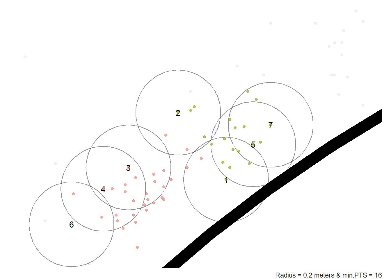
Figure 10.2: Close up look at the DBSCAN algorithm

As you can see from Figure 10.2, shot 1 only has 10 core points while shot 2 has 7 core points. We know that the number of core points need to be greater than or equal to the minPTS parameter for a shot to be added to the cluster. Let's increase \(\varepsilon\) or decrease minPTS as an attempt to merge these two clusters together. It is very unlikely that players voluntarily took shots in two spots just a few feet apart. It's much more likely that the two clusters are a result of luck and measurement error⁷¹.

10.1.4 Tuned Results

After a few trying a few different combinations, it seems that \(\varepsilon = 0.3\) and minPTS\(= 15\) gave the resulted in more useful results⁷².

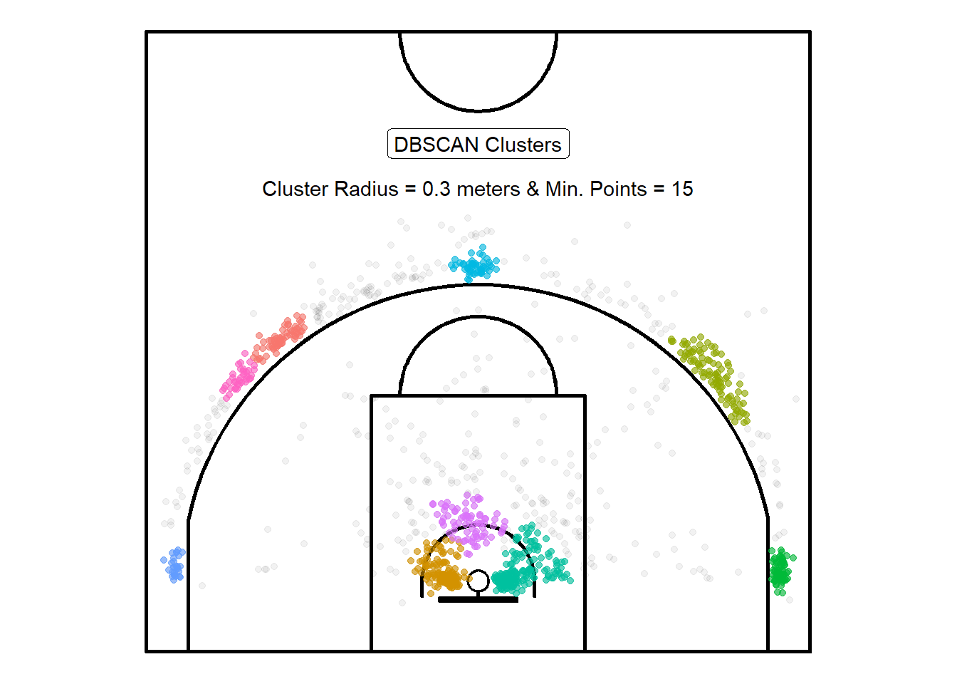
Figure 10.3: Bigger clusters but still two separate ones on the top right

We can delimit the perimeter of our clusters by connecting the exterior points of our clusters. The technical term for this is to create a convex hull around the clusters. The following analogy might be useful to better understand this concept. Think of the basketball court as a cork bulletin board. Now imagine that we placed colour-coded pins at the locations of the exterior shots of each cluster. The convex hull would be like placing an elastic around the pins of the same colour. This can easily be achieved using the st_convex_hull() function from the sf package.

# Convert shots to an sf object
hull_sf <- clusters_sf %>% 
  group_by(cluster_id) %>%
  summarise(geometry = st_combine(geometry)) %>%
  st_convex_hull()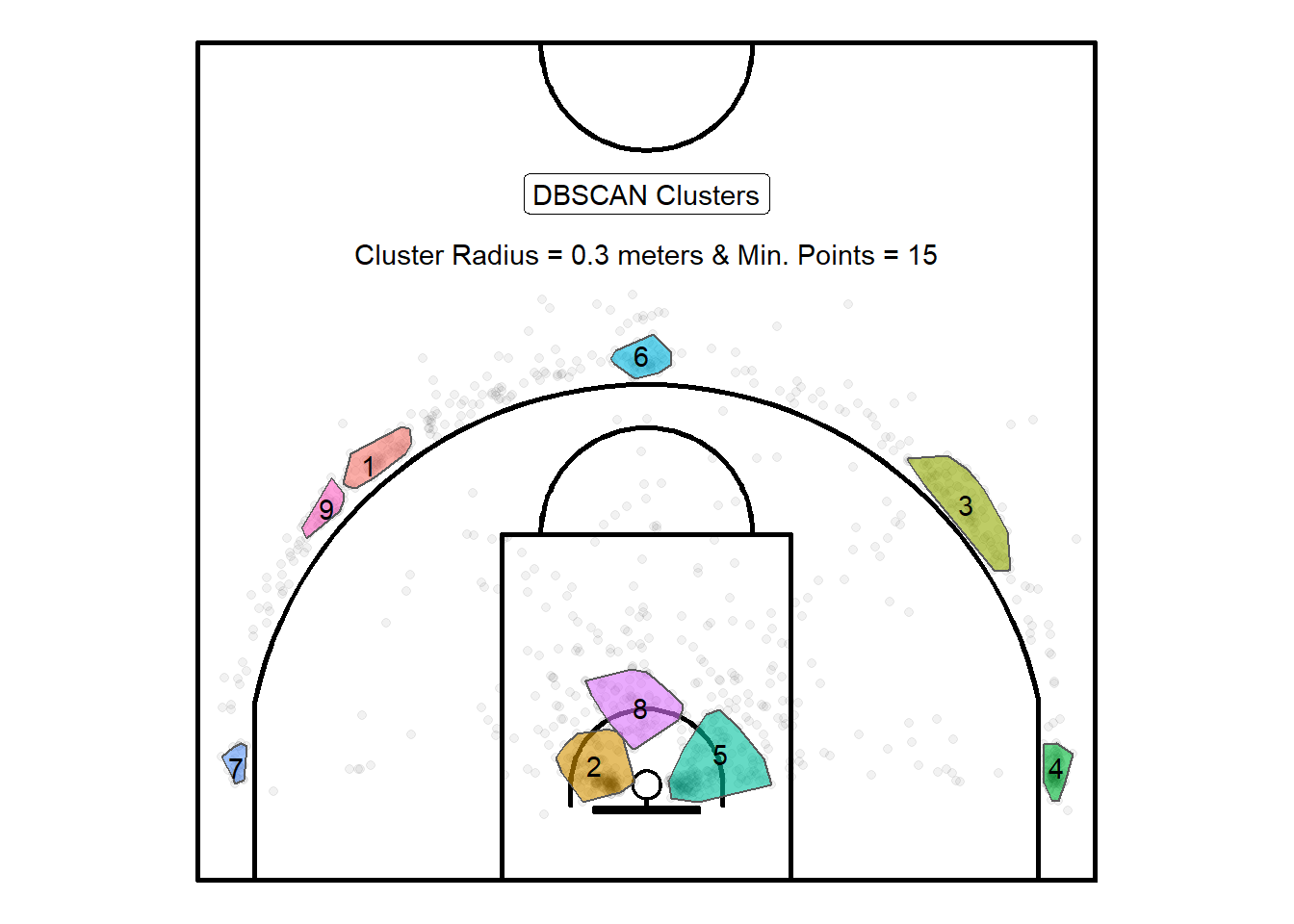

Figure 10.4: Try to visualize the pins and elastic analogy

We can see from Figure 10.4 that the algorithm settled with 9 clusters with the new parameters. Cluster 9 and cluster 1 represent almost certainly the same true underlying pattern. If they would merge, then they would look similar to cluster 3 which is more representative of the signal. The clusters are larger as a result of the more generous initial parameters⁷³. Additionally, cluster 8 is a cluster that makes sense in terms of common shot locations.

10.2 Further Investigation

HDBSCAN is an extension of DBSCAN. A key difference between the two algorithms is that only the minPTS parameter needs to be specified for HDBSCAN.

# Convert the shots sf object to a dataframe with the xy-coordinates
hdb <- hdbscan(shots_df, minPts = min_points)

# Create an sf object with the shots and cluster ID
clusters_sf <- st_as_sf(
  x = shots_sf %>% 
    mutate(cluster_id = hdb$cluster) %>%
    filter(cluster_id >= 1)
  )

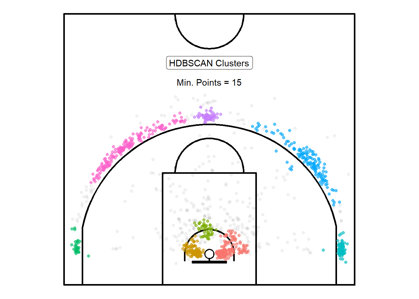
Figure 10.5: Points leaking past the three-point line

Figure 10.5 displays the results of HDBSCAN with minPTS\(= 15\). It appears that some of the long mid-range shots were lumped in the three-point clusters. We could try to improve the clustering performance by feeding the algorithm other numeric information such as whether the shot was worth two or three points, the shot distance, and the shot angle in addition to only using the shot coordinates⁷⁴. Lastly, it might be useful to apply this clustering technique to individual player's shots. We could try to compare where different players shoot from and see it the cluster locations match the strategy implemented by the coaching staff.

The next chapter will build on the ideas proposed in this chapter. Instead of trying to classify shots into clusters, we will try to calculate a density value for every spot on the court to see where the shots are coming from through another lens. Finally, the next chapter will attempt to find spots on the court where the players in the sample were the most accurate.

Note that all the R code used in this book is accessible on GitHub.

9 Nearest Neighbour Analysis

11 The Landscape of Modern Basketball