6 Dividing the Court into Zones

Note that all the R code used in this book is accessible on GitHub.

There are many ways to split up a basketball court into zones. For this reasons, we will match the way that the NBA does it⁴².

6.1 Basic Zones

Let's create sf polygons for these zones to later conduct some spatial analysis. Creating these polygons is very similar to what we've done in Chapter 5 so we'll focus on the zones themselves instead of focusing on the code.

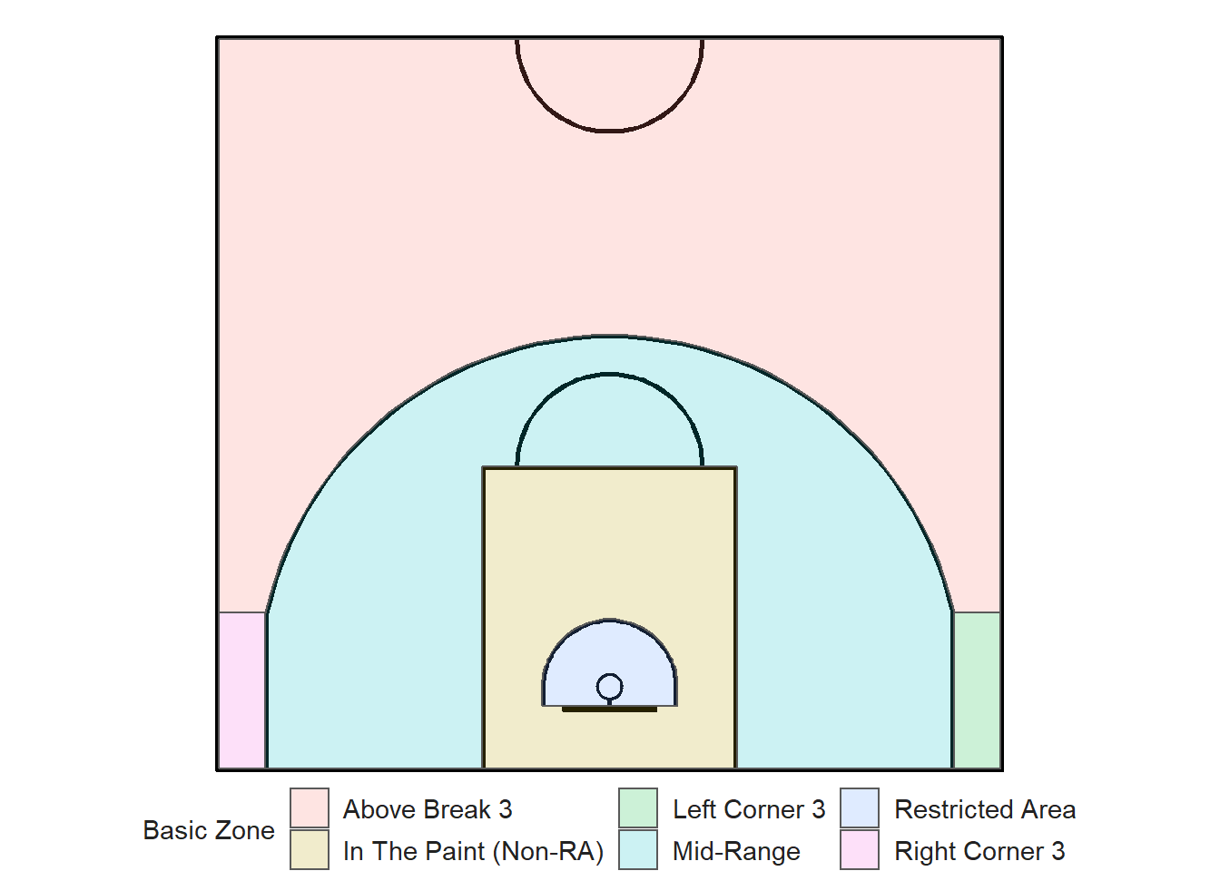
Figure 6.1: Basic zones for FIBA basketball court

As you can see from the picture above, the basic zones are mutually exclusive and cover the entirety of the half-court. Thus, each shot could be assigned a basic zone using the st_join() function from the sf package. From there, it is easy to calculate summary statistics for each zone.

6.2 Point Value

We can also create polygons for the two areas with different point values.

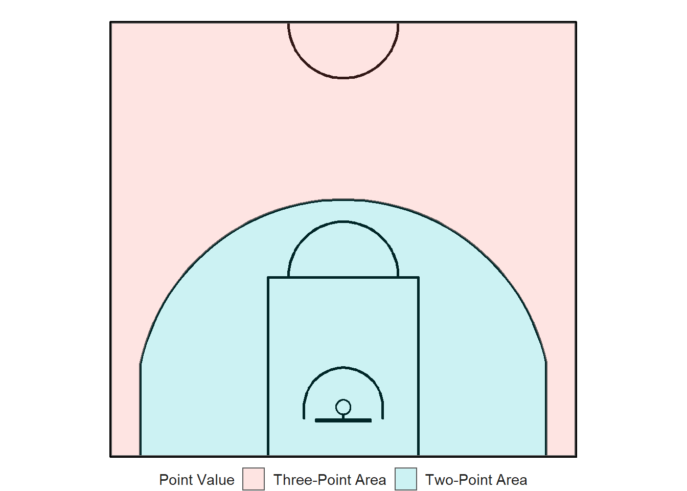
Figure 6.2: Point-value zones for FIBA basketball court

This is useful since the three-point and two-point shot attempts are considered for the field goal percentage⁴³. Knowing the point-value of each shot is crucial to calculate the effective field goal percentage which adjusts for the fact that a 3-point field goal is worth one more point than a 2-point field goal.

6.3 Shot Distance

Next, we can separate the court into zones based on distance.

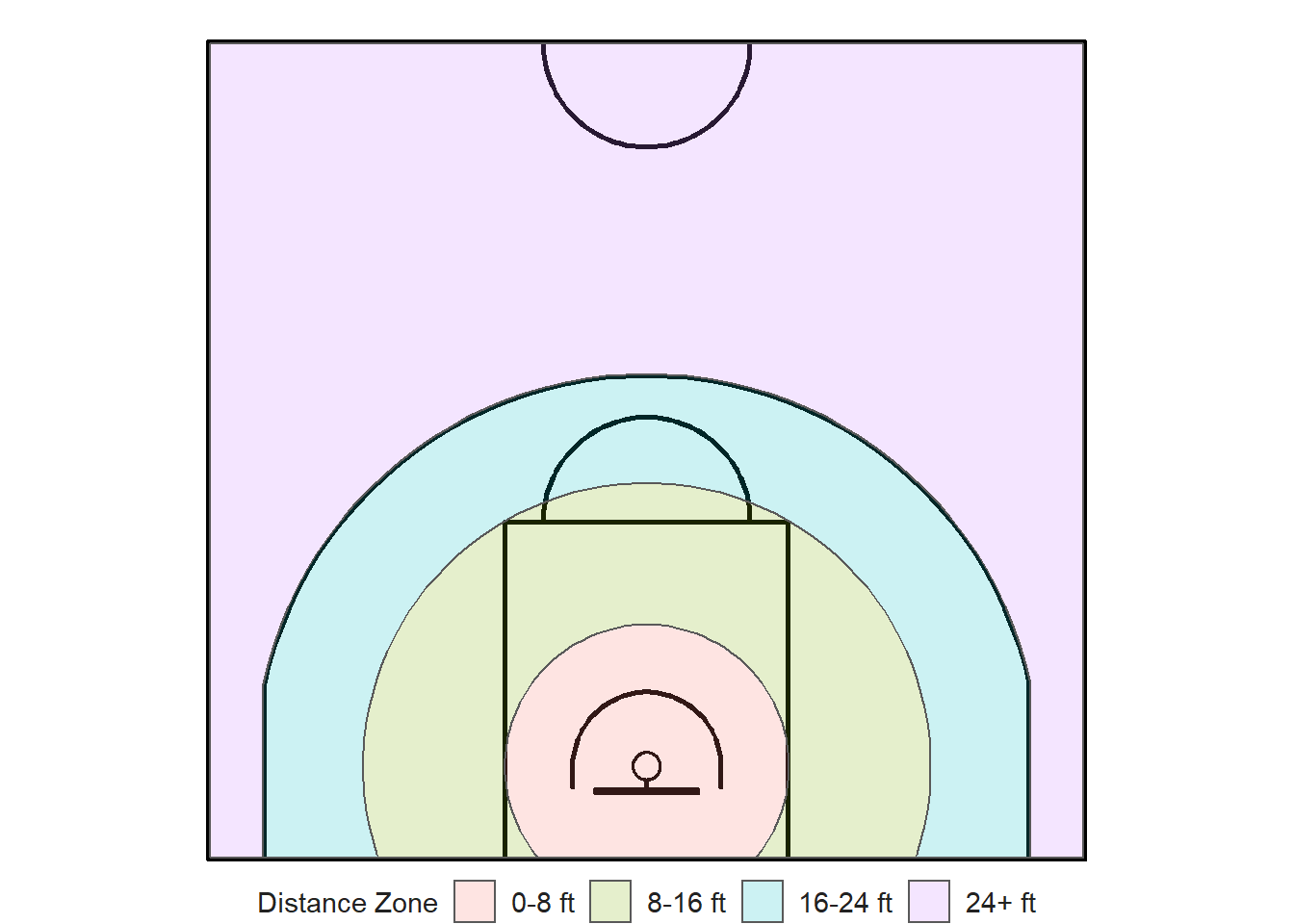
Figure 6.3: Distance zones for FIBA basketball court

We know that the distance from the hoop has a significant effect on the probability of making a shot. Being able to easily bin your shots by distance is crucial.

6.4 Shot Angle

Lastly, we can split the court by angle. We want to have the following zones:

• Left Side
• Left Center
• Center
• Right Center
• Right Side

There are many ways to separate the court into these 5 zones based on angle. We need to choose two arbitrary lines that go through the center of the hoop. Let's pick the lines that pass the exterior corner of the top key⁴⁴ and the top exterior point of the straight part of the three-point line⁴⁵.

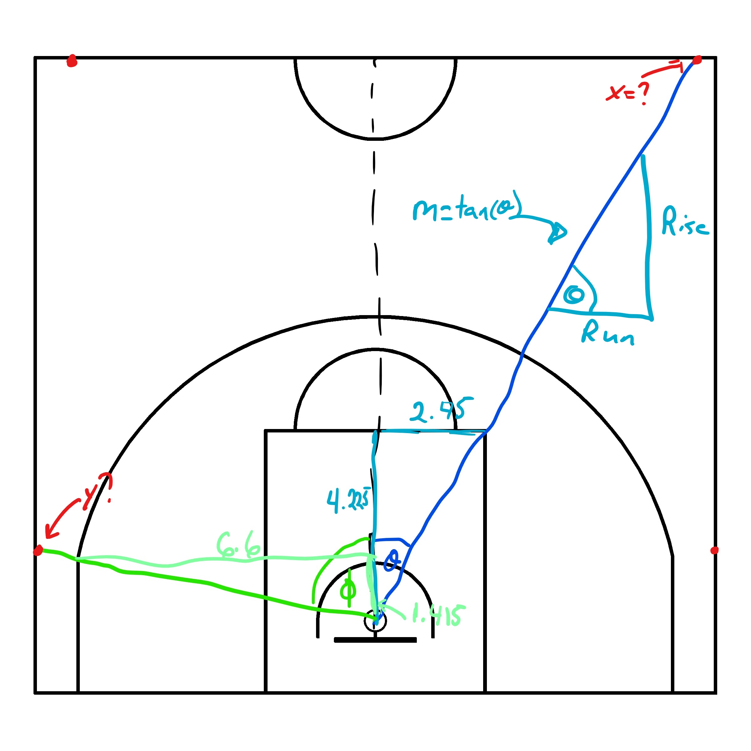
Figure 6.4: Choice of arbitrary lines to divide the court by angle

Finding the \((x, ~y)\) coordinates of the red dots in Figure 6.4 can be challenging. We can calculate \(\theta\) and \(\phi\) by using SOH CAH TOA. Since we have the measures for the adjacent and opposite sides of each angles, we will use the tangent trigonometric ratio (TOA). We get that \(\theta = \arctan{\frac{O}{A}} \approx 30^{\circ}\) and \(\phi \approx 78^{\circ}\).

We know any line has equation \(y = mx + b\). We also know that the slope of a line can be represented as \(tan(\theta)\) where \(\theta\) is the angle from the horizontal. That said, we have \(y = \tan{(\theta)}x + b\). We know that the center of the hoop lies on both lines so we can substitute \(x\) and \(y\) in each line equation with \((7.5, ~1.575)\) to solve for the y-intercepts \(b\). The coordinates of the red dots can now be easily identified once we know the line equations and one of their components.

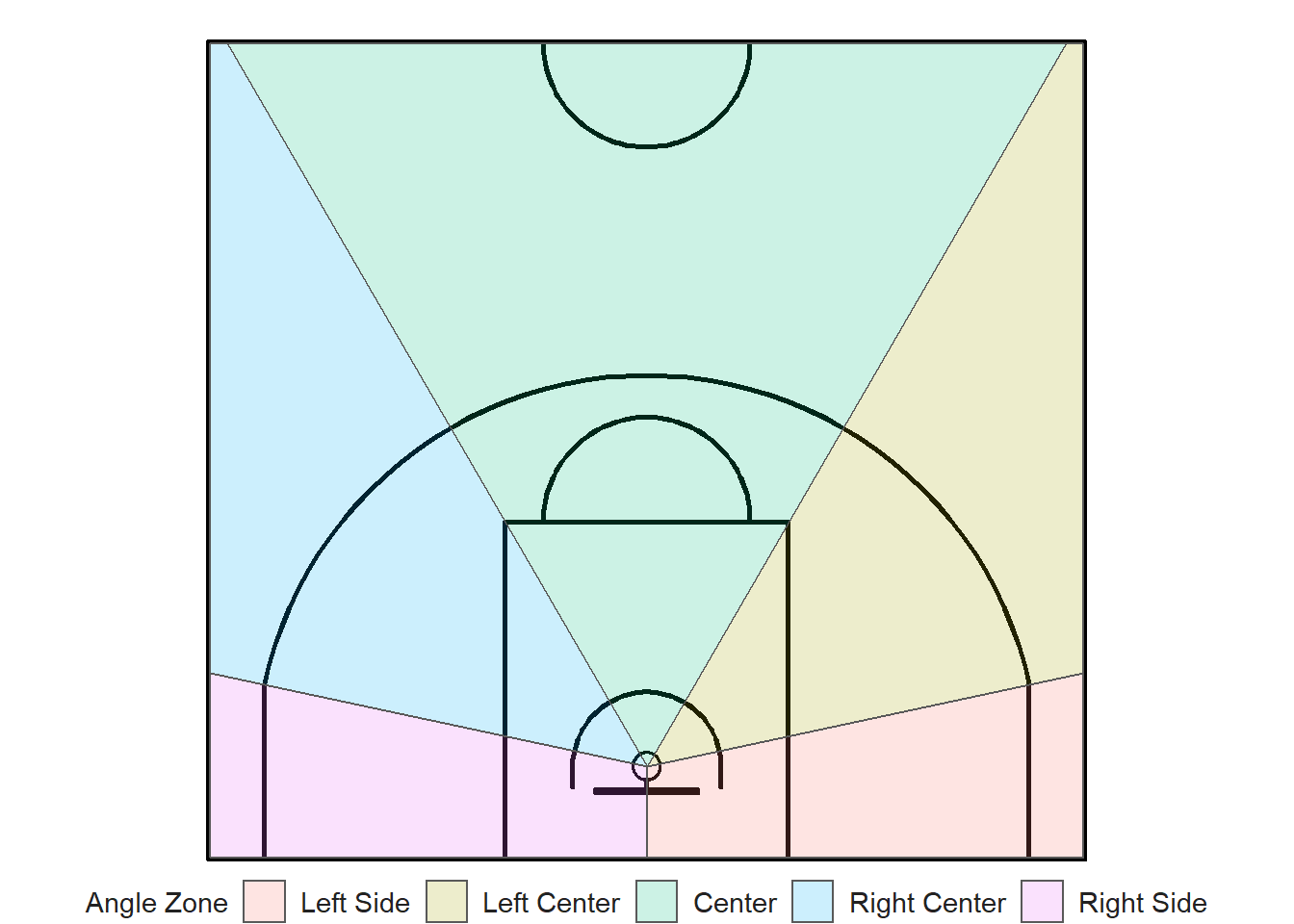
Figure 6.5: Angle zones for FIBA basketball court

We will see in the next chapter how we can use these zone polygons to create an augmented spatial basketball shots data set.

Note that all the R code used in this book is accessible on GitHub.