13 Quantifying Shooting Ability

Note that all the R code used in this book is accessible on GitHub.

We will use our GAM models from the previous chapter to try separate a player's ability to make shots from the quality of the shots the are taking. This line of thinking was heavily influenced by Yu-Han Chang et al.'s paper Quantifying Shot Quality in the NBA. In our case, we will define shot quality as the number of points the average player in the sample can expect for a specific shot.

We can use our model that only considered the location of the shot to predict the probability of a made shot for a specific location. The expected points per shots can then be obtained by multiplying the probability by the number of points the shot would generate⁹⁰.

# GAM model based on shot coordinates
coord_mod <- gam(
  shot_made_numeric ~ s(loc_x, loc_y),
  data = near_shots, method = "REML", family = binomial)

Table 13.1: Expected Points as a measure of shot quality

dist_feet	shot_value	make_prob	x_points	actual_points
3.422	2	0.464	0.929	0
24.705	3	0.408	1.225	0
1.748	2	0.623	1.247	2
2.651	2	0.594	1.187	2
2.695	2	0.520	1.041	2
23.840	3	0.372	1.117	3
5.110	2	0.391	0.782	0
23.421	3	0.383	1.149	0
10.654	2	0.449	0.899	0
8.745	2	0.325	0.650	2

Table 13.1 displays the make probability and expected points per shot predicted by the coordinate-only model.

We know that the Effective Field Goal Percentage of a player can be calculated by using the formula below:

\[ \mbox{EFG} = \frac{2FG + 1.5 \times 3FG}{FGA}, \]

where \(2FG\) is number of made shots from the two-point area, \(3FG\) is number of made shots from the three-point area, and \(FGA\) is the number of shots a player took.

We will define a player's shot quality (SQ) as their Predicted Effective Field Goal Percentage. We can multiply the entries of the make_prob column by the \(1.5\) for the three-point shots and average the new weighted make_prob column to get a player's SQ score.

\[ \mbox{SQ} = \frac{\sum_{i=1}^{FGA}w_i}{FGA}, \]

where \(w_i\) is equal to the make_prob of shot \(i\) for two-pointers and \(w_i = 1.5 \times \mbox{make_prob}_i\) for three-pointers. In other words, \(w_i\) is the weighted make probability of a specific shot or the effective field goal percentage of a shot taken by the average player in the sample. Thus, SQ if the effective field goal percentage that the average player would get if they took the same shots. That said, if the player's EFG is greater than their SQ, this implies that they shot better than predicted by the GAM model; that they shot better than the average player.

Thus, we can define a player's shot making abilities (SM) as

\[ \mbox{SM} = \mbox{EFG} - \mbox{SQ} \]

since = + . We can think of SM as a measure of how much better or worse the player shot compared to the average player taking the same shots. A positive SM indicates that the player shot better than expected.

Table 13.2: Voila! Who are the best shot makers?

player	position	shot_attempts	efg	esq	esm
Player 14	Guard	455	58.5	48.9	9.6
Player 13	Guard	409	58.1	50.7	7.4
Player 15	Guard	54	50.0	53.4	-3.4
Player 7	Guard	295	49.3	49.3	0.0
Player 4	Post	169	57.7	50.1	7.6
Player 12	Post	82	48.2	45.5	2.7
Player 16	Post	35	62.9	53.7	9.2
Player 5	Guard	117	47.9	46.7	1.1
Player 11	Guard	327	45.4	47.5	-2.1
Player 19	Post	6	50.0	42.4	7.6
Player 17	Post	120	56.7	52.3	4.3
Player 8	Guard	83	35.5	49.9	-14.3
Player 3	Guard	189	41.5	46.8	-5.3
Player 9	Post	61	42.6	48.1	-5.4
Player 10	Post	201	40.0	51.6	-11.5
Player 18	Guard	65	30.8	51.0	-20.3
Player 6	Guard	48	32.3	50.9	-18.6
Player 2	Post	53	36.8	46.4	-9.6
Player 1	Post	55	45.5	54.8	-9.4

The SM and SQ values for each player are summarized in Table 13.2. By definition, adding the values of the SM and SQ columns result in the values of the EFG column. The results of Table 13.2 are most likely easier to digest when visualized in Figure 13.1 below.

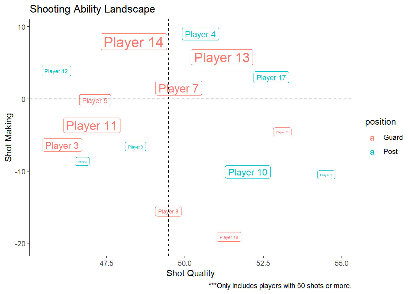
Figure 13.1: What do the four quadrants mean?

The Shot Quality (SQ) is displayed on the \(x\)-axis. Low values for shot quality (left) indicates that the player is taking difficult shots⁹¹. High values of shot quality (right) indicates that the player is taking easier shots in terms of location. The vertical dashed line represents the average shot quality.

Shot Making (SM) is displayed on the \(y\)-axis. Values above the horizontal dashed line indicate that the player is shooting better than expected. Low values of shot making indicate an underperformance relative to their expectation. The player labels are scaled by the number of shots attempted by the players.

The players in the top-left quadrant of Figure 13.1 are taking the toughest shots in terms of location and still manage to make them way above expectation. The players in the bottom-right quadrant are shooting from regions that the average player would generate the most points per shot but struggle to shoot better than this average player.

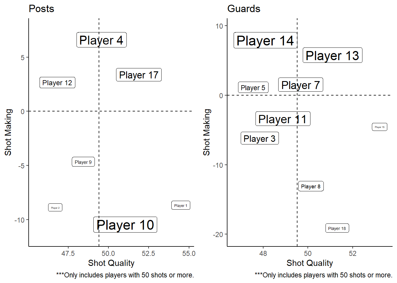
Figure 13.2: Comparing apples to apples (ish)

Figure 13.2 separates Figure 13.1 into two plots according to the positions of the players. This can help better compare similar players competing for a similar role in the lineup.

Of course, there are many other variable that influence whether a shot is difficult or not other than the \((x, ~y)\) coordinates of the shot. Defender distance is an obvious variable that is not included in our coordinate-only GAM model that would improve the validity of the results. That said, the goal of this chapter was to lay out the conceptual framework behind shooter evaluation that goes beyond simply comparing effective field goal percentages.

Note that all the R code used in this book is accessible on GitHub.