7 Basketball Shots as Spatial Objects

Note that all the R code used in this book is accessible on GitHub.

Let's load the basketball court and spatial polygons we've built in the previous chapters.

# Load the plot_court() function from the previous chapters
source("code/court_themes.R")
source("code/fiba_court_points.R")
# Load the different zone polygon objects
source("code/zone_polygons.R")

# Load libraries
library(tidyverse) # ggplot and dplyr
library(sf) # working with spatial objects

Next, we can load the augmented basketball shots data set we created in Chapter 2.

# Load shot data
shots <- readRDS(file = "data/shots_augmented.rds")

Table 4.4: Display the first few shots of augmented data

player	loc_x	loc_y	shot_made_factor	dist_feet	theta_deg
Player 7	4.39	7.96	Make	23.29	26.01
Player 3	5.78	8.51	Miss	23.44	13.93
Player 7	3.00	7.08	Make	23.33	39.23
Player 3	3.38	7.20	Miss	22.89	36.22
Player 13	3.16	7.20	Miss	23.31	37.63
Player 7	3.33	7.14	Miss	22.82	36.84

Note that we have access to who took the shot, whether they made it or not, and from where on the court they released it. From there, we used the Pythagorean theorem to calculate the shot distance from the center of the hoop and we used trigonometric ratios to calculate the angle from the center line.

7.1 The Spatial Advantage

We can convert our augmented shot data to an sf object to take advantage of the spatial nature of the data.

# convert shots to an sf object
shots_sf <- st_as_sf(shots, coords = c("loc_x", "loc_y"))

# View sf object
shots_sf %>% select(-shot_made_numeric, -dist_meters, -theta_rad)

## Simple feature collection with 1163 features and 4 fields
## Geometry type: POINT
## Dimension:     XY
## Bounding box:  xmin: 0.366552 ymin: 1.072896 xmax: 14.71044 ymax: 9.802368
## CRS:           NA
## # A tibble: 1,163 x 5
##    player    shot_made_factor dist_feet theta_deg            geometry
##    <fct>     <fct>                <dbl>     <dbl>             <POINT>
##  1 Player 7  Make                 23.3       26.0  (4.386864 7.95528)
##  2 Player 3  Miss                 23.4       13.9   (5.7798 8.510016)
##  3 Player 7  Make                 23.3       39.2 (3.003072 7.083552)
##  4 Player 3  Miss                 22.9       36.2 (3.377976 7.202424)
##  5 Player 13 Miss                 23.3       37.6 (3.161568 7.202424)
##  6 Player 7  Miss                 22.8       36.8 (3.329208 7.141464)
##  7 Player 7  Make                  2.01      82.2  (6.89232 1.658112)
##  8 Player 7  Make                 23.2       39.4 (3.009168 7.050024)
##  9 Player 11 Make                 23.3       38.8   (3.05184 7.10184)
## 10 Player 18 Miss                 22.6       37.2 (3.344448 7.059168)
## # ... with 1,153 more rows

The simple fact that our shots dataframe is now an sf object means that we can use the st_join() function which will automatically create zone columns based on the location of each shot relative to the polygons we created in Chapter 6.

# shot_zone_range
shots_sf <- st_join(
  x = shots_sf,
  y = distance_polys
) %>%
  # shot_zone_area
  st_join(
    y = angle_polys
  ) %>%
  # shot_zone_basic
  st_join(
    y = basic_polys
  ) %>%
  # area_value
  st_join(
    y = point_polys
  ) %>%
  # shot_value
  mutate(
    shot_value = ifelse(area_value == "Two-Point Area", 2, 3)
  ) %>%
  # Reorder and only keep relevant variables
  select(player, shot_made_numeric, shot_made_factor,
         dist_feet, dist_meters, theta_deg, theta_rad, shot_value,
         shot_zone_range, shot_zone_area, shot_zone_basic, area_value,
         geometry)

The easiest way to test whether the join worked properly would be to randomly select a few shots and plot their different zone labels.

set.seed(123) # Always Display the same random shots
sample_shots_sf <- shots_sf %>% 
  # Randomly select 20 shots
  slice_sample(n = 20)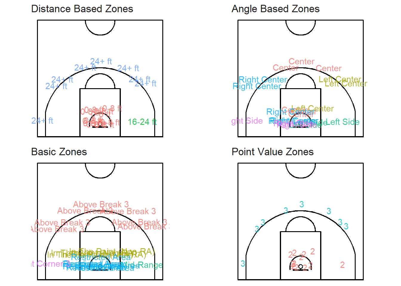

Figure 5.5: Check labels for the same20 random shots

It seems like our joins worked properly. Let's save this new data set so we can easily load it in future chapters.

# Save the spatial data
saveRDS(shots_sf, file = "data/shots_sf.rds")

In the next chapter, we will create our first shot chart. How exciting! More specifically, we will try to determine whether the shot locations are spatially randomly distributed or if they seem to cluster.

Note that all the R code used in this book is accessible on GitHub.