5 Building a Basketball Court in R

Note that all the R code used in this book is accessible on GitHub.

We chose to use the sf package to plot a basketball court instead of simply using ggplot2 because the sf was built to work with polygons and spatial data. The two packages work hand in hand. First, we'll use sf to generate the court points based on the FIBA court dimensions⁴¹. Second, we'll write the plot_court() function to easily plot a basketball court using ggplot2 moving forward. This chapter was heavily influenced by Todd W. Schneider's Ballr Shiny app.

5.1 Generating the Court Points

5.1.1 Official Dimensions

Let's use these two images taken from an official FIBA document to get some basic dimensions. Note that all lengths are measured in meters.

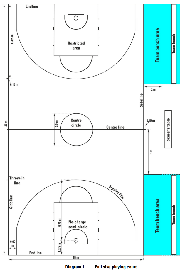
Figure 5.1: Full FIBA court dimensions

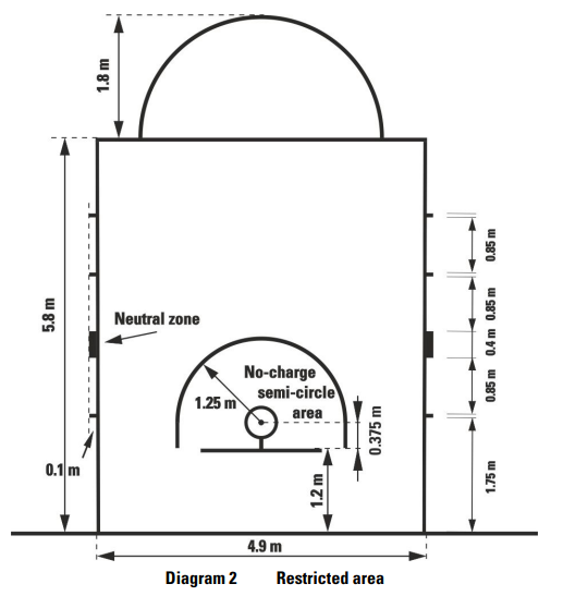
Figure 5.2: FIBA court key dimensions

# Load the libraries
library(sf) # Work with polygons
library(tidyverse) # ggplot2 and dplyr 

# Load some predefined court themes for the plot_court() functions
# Code found at https://github.com/olivierchabot17/ballbook
source("code/court_themes.R")

# All lengths will be in meters
line_thick = 0.05
width = 15
height = 28 / 2
key_height = 5.8
key_width = 4.9
key_radius = 1.8
backboard_width = 1.8
# https://www.fiba.basketball/documents/BasketballEquipment.pdf
backboard_thick = 0.1
backboard_offset = 1.2
hoop_radius = 0.45 / 2
hoop_center_y = 1.575
rim_thick = 0.02
neck_length = hoop_center_y - (backboard_offset + hoop_radius + rim_thick)
three_point_radius = 6.75
three_point_side_offset = 0.9
three_point_side_height = sqrt(
  three_point_radius^2 - (three_point_side_offset - width/2)^2
  ) + hoop_center_y
restricted_area_radius = 1.25

5.1.2 Half-Court

Once we have defined a few basic dimensions, we can proceed to create polygons for each of the lines. For now, we will only build a half-court since that's what's needed to create shot charts. However, building the full court would be fairly simple to accomplish using the same approach.

This vignette provides a few examples of creating polygons using the sf package. Recall the coordinate system we defined in Chapter 2.

The origin was placed at the bottom-left corner of the half-court from our perspective. Note that the \((0, ~0)\) is placed at the interior of the half-court and that all lines are 5 centimeters thick. Therefore, the interior of the half-court has a base of 15 meters and a height of 14 meters. The exterior of the half-court is 15.1 meters wide and 14.1 meters high as a result of the 0.05 meters width of each line. We chose to define the lines as a polygon within a polygon using the st_polygon() function to prevent the ambiguity of letting the plotting software decide on the line width. This way, we can be confident that the court appearing on the screen reflects the true dimensions.

For convention, we can list the vertices of the polygons starting from the bottom-left and move clockwise from there.

# Draw a rectangle that defines the half-court interior
half_court_int <- rbind(
  c(0, 0),
  c(0, height),
  c(width, height),
  c(width, 0),
  c(0,0)
  )

# Draw a rectangle that defines the half-court exterior
half_court_ext <- rbind(
  c(0-line_thick, 0-line_thick),
  c(0-line_thick, height + line_thick),
  c(width + line_thick, height + line_thick),
  c(width + line_thick, 0-line_thick),
  c(0-line_thick, 0-line_thick)
  )

# Define a sfg polygon object in sf by subtracting interior from exterior
half_court <- st_polygon(list(half_court_ext, half_court_int))

# Verify sfg class of polygon
class(half_court)

## [1] "XY"      "POLYGON" "sfg"

# Plot the half-court rectangle to test our object
ggplot() +
  geom_sf(data = half_court) +
  theme_classic() +
  scale_x_continuous(breaks = seq(from = 0, to = 15, by = 3))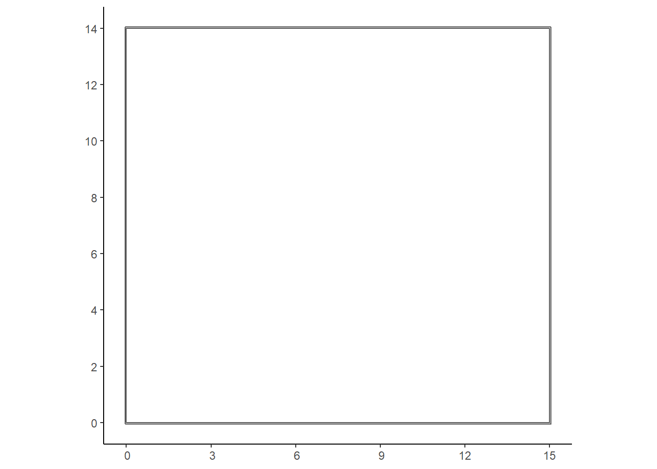

5.1.3 Other Rectangles

We see that the rectangle above the width and height of the half-court are indeed 15 and 14 meters respectively. We can repeat this process for all rectangular objects in the half-court.

# Draw a rectangle for the key
key_int <- rbind(
  c(width/2 - key_width/2 + line_thick, 0),
  c(width/2 - key_width/2 + line_thick, key_height - line_thick),
  c(width/2 + key_width/2 - line_thick, key_height - line_thick),
  c(width/2 + key_width/2 - line_thick, 0),
  c(width/2 - key_width/2 + line_thick, 0)
)

key_ext <- rbind(
  c(width/2 - key_width/2, 0),
  c(width/2 - key_width/2, key_height),
  c(width/2 + key_width/2, key_height),
  c(width/2 + key_width/2, 0),
  c(width/2 - key_width/2, 0)
)

key <- st_polygon(list(key_ext, key_int))

# Draw a rectangle for the backboard
backboard_points <- rbind(
  c(width/2 - backboard_width/2, backboard_offset - backboard_thick),
  c(width/2 - backboard_width/2, backboard_offset),
  c(width/2 + backboard_width/2, backboard_offset),
  c(width/2 + backboard_width/2, backboard_offset - backboard_thick),
  c(width/2 - backboard_width/2, backboard_offset - backboard_thick)
)

backboard <- st_polygon(list(backboard_points))

# Neck
neck_points <- rbind(
  c(width/2 - line_thick/2, backboard_offset),
  c(width/2 - line_thick/2, backboard_offset + neck_length),
  c(width/2 + line_thick/2, backboard_offset + neck_length),
  c(width/2 + line_thick/2, backboard_offset),
  c(width/2 - line_thick/2, backboard_offset)
)

neck <- st_polygon(list(neck_points))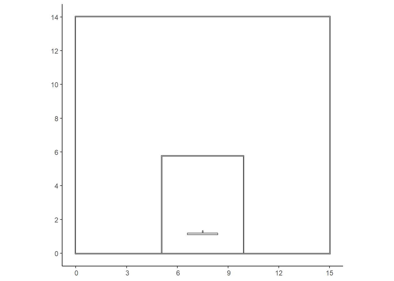

Figure 5.3: Plot all the rectangular objects

5.1.4 Hoop

Now we can use the st_point() function from the sf package to define an sfg point object located at the center of the hoop \((7.5, ~ 1.575)\). The st_buffer() function creates a padding of a specified distance around a spatial object. In this case, we set the dist argument to the radius of a FIBA basketball rim which is 22.5 centimeters. We set the rim thickness to 2 centimeters so the exterior of the rim has a radius of \(22.5 + 2 = 24.5\) centimeters. Lastly, we can test our new circular polygon by plotting it in orange.

# Define a point sfg object for the center of the hoop
hoop_center <- st_point(c(width/2, hoop_center_y))

# Check class of hoop_center
class(hoop_center)

## [1] "XY"    "POINT" "sfg"

# Interior of the rim
# Buffer the point by the radius of the hoop to create a circle
hoop_int <- hoop_center %>%
  st_buffer(dist = hoop_radius)

# Exterior of the rim
hoop_ext <- hoop_center %>%
  st_buffer(dist = hoop_radius + rim_thick)

# Subtract interior from exterior to get the rim
hoop <- st_polygon(list(
  # Only kepp the X, Y columns of the coordinates
  st_coordinates(hoop_ext)[ , 1:2],
  st_coordinates(hoop_int)[ , 1:2]
  ))

# Check class of hoop object
class(hoop)

## [1] "XY"      "POLYGON" "sfg"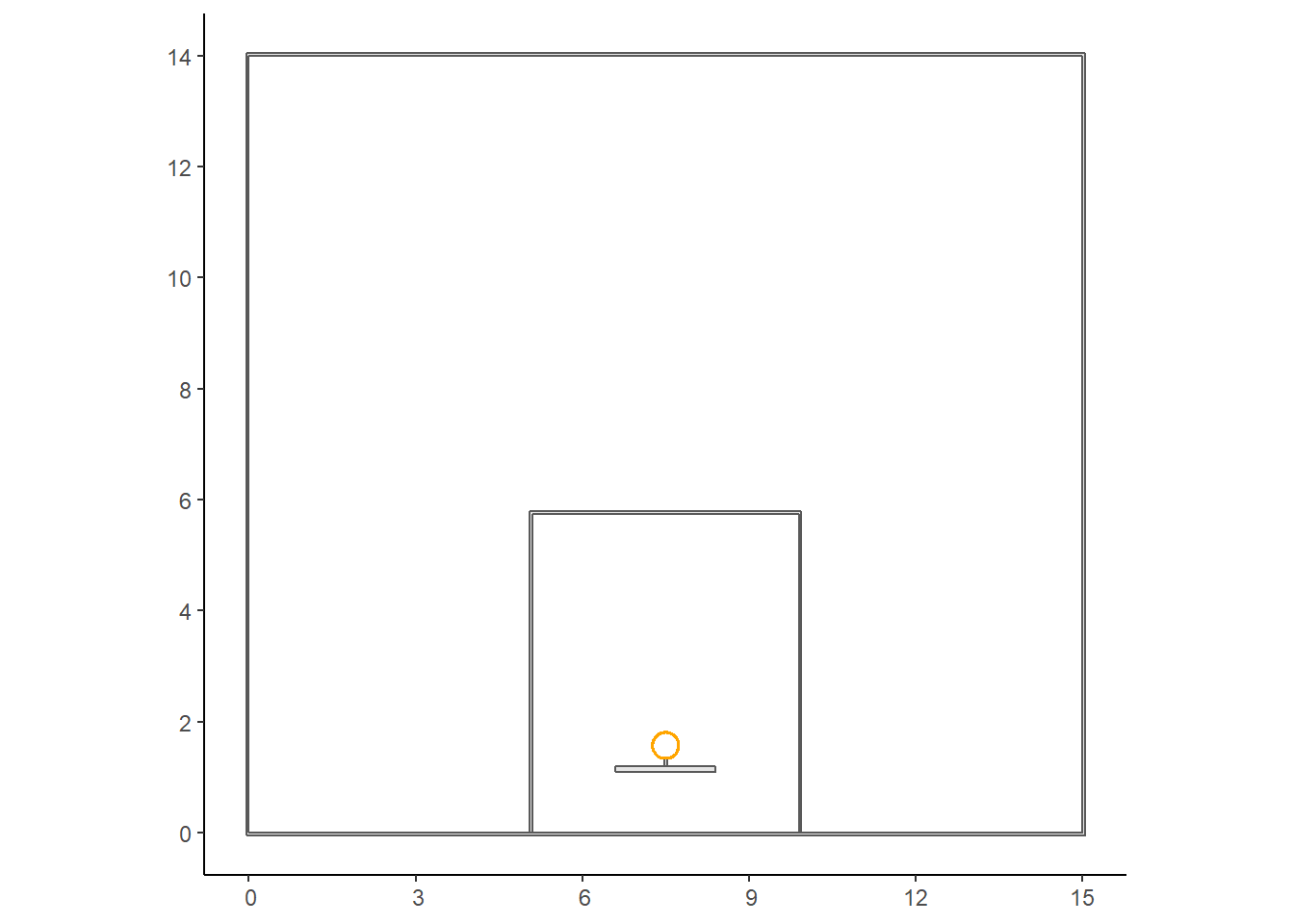

Figure 5.4: Adding the hoop in orange

5.1.5 Semi-Circles

We can plot the semi circles at the top of the key and at the half-court by cutting our full circle in half using the st_crop() function.

# Draw the half-circle at the top of the key
key_center <- st_point(c(width/2, key_height))

key_circle_int <- st_crop(
  st_sfc(st_buffer(key_center, dist = key_radius - line_thick)),
  # Only keep the part of the circle above the top of the key
  xmin = 0, ymin = key_height, xmax = width, ymax = height
  )

key_circle_ext <- st_crop(
  st_sfc(st_buffer(key_center, dist = key_radius)),
  xmin = 0, ymin = key_height, xmax = width, ymax = height
)

key_circle <- st_polygon(list(
  st_coordinates(key_circle_ext)[ , 1:2],
  st_coordinates(key_circle_int)[ , 1:2]
  ))

# Draw the half-circle at the bottom of half-court
half_center <- st_point(c(width/2, height))

half_circle_int <- st_crop(
  st_sfc(st_buffer(half_center, dist = key_radius - line_thick)),
  # only keep the bottom half below the half-court line
  xmin = 0, ymin = 0, xmax = width, ymax = height
)

half_circle_ext <- st_crop(
  st_sfc(st_buffer(half_center, dist = key_radius)),
  xmin = 0, ymin = 0, xmax = width, ymax = height
)

half_circle <- st_polygon(list(
  st_coordinates(half_circle_ext)[ , 1:2],
  st_coordinates(half_circle_int)[ , 1:2]
))

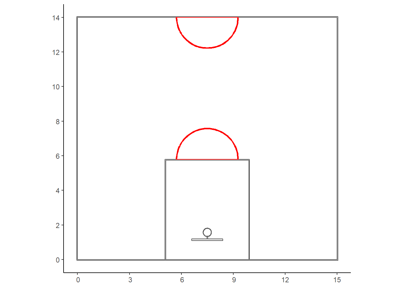
Figure 5.5: Adding the red semi-circles

5.1.6 Three-Point Line

We are only missing the three-point line and the line for the restricted area. These polygons are slightly more challenging since they are circles connected to straight lines. We know from Figure 5.1 that the exterior of the vertical parts are 0.9 meters from the edge of the court. Furthermore, we know that the circular part of the three-point line is centered around the center of the rim and has a radius of 6.75 meters. Note that the general equation of a circle is \((x-x_0)^2 + (y-y_0)^2 = r^2\), where \((x_0, ~y_0)\) are the coordinates of the center of the circle. Thus, the full circle equation of the three-point line given our reference system is \((x - 7.5)^2 + (y - 1.575)^2 = 6.75^2\). This equation can be rearranged as \(y = \pm \sqrt{6.75^2 - (x - 7.5)^2} + 1.575\). Let's only consider \(f(x) = \sqrt{6.75^2 - (x - 7.5)^2} + 1.575\) since the three-point line represents the upper half of the circle. Since we know that the \(x\) values of the vertical lines are \(x_1 = 0.9\) and \(x_2 = 15 - 0.9 = 14.1\), we can find the \(y\) values to crop our circle at. The points of intersect are at

\[ f(0.9) = \sqrt{6.75^2 - (0.9 - 7.5)^2} + 1.575 = 2.99 ~ \mbox{meters.} \]

It might be easier to viusalize the problem using this desmos graph printed below.

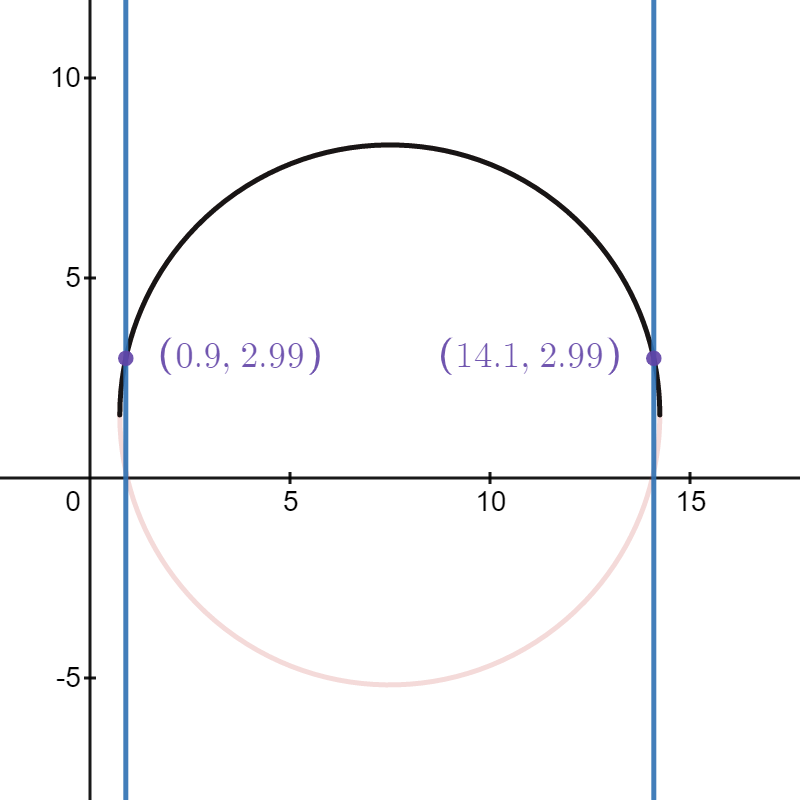
Figure 5.6: Finding the points of intersection of the three-point line

In short, we need to crop the three-point circle at 2.99 meters and bind these points to the points on the straight lines on each side of the three-point line.

# Define a point sfg object for the center of the hoop
three_center <- st_point(c(width/2, hoop_center_y))

# Buffer the point to create a circle & crop it at 2.99 meters
three_int <- st_crop(
  st_sfc(st_buffer(three_center, dist = three_point_radius - line_thick)),
  xmin = three_point_side_offset + line_thick, ymin = three_point_side_height,
  xmax = width - (three_point_side_offset + line_thick), ymax = height
)

# Get the number of rows of coordinates of the three_int object
n <- nrow(st_coordinates(three_int))

# Bind the straight line points to the arc
three_int <- rbind(
  c(three_point_side_offset + line_thick, 0),
  c(three_point_side_offset + line_thick, three_point_side_height),
  # Remove the last two rows and only keep the X,Y columns
  st_coordinates(three_int)[1:(n-2), 1:2],
  c(width - (three_point_side_offset + line_thick), three_point_side_height),
  c(width - (three_point_side_offset + line_thick), 0),
  c(three_point_side_offset + line_thick, 0)
)

# Do the same for the exterior
three_ext <- st_crop(
  st_sfc(st_buffer(three_center, dist = three_point_radius)),
  xmin = three_point_side_offset, ymin = three_point_side_height,
  xmax = width - three_point_side_offset, ymax = height
)

three_ext <- rbind(
  c(three_point_side_offset, 0),
  c(three_point_side_offset, three_point_side_height),
  st_coordinates(three_ext)[1:(n-2), 1:2],
  c(width - three_point_side_offset, three_point_side_height),
  c(width - three_point_side_offset, 0),
  c(three_point_side_offset, 0)
)

# Create a three-point line sfg polygon object
three_point_line <- st_polygon(list(three_int, three_ext))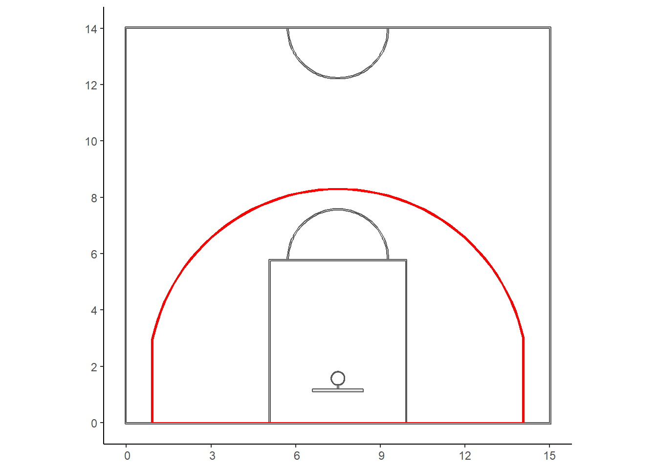

Figure 5.7: Plotting the three-point line in red

5.1.7 Restricted Area

The same approach can be used to create a spatial object for the restricted area. There are two key differences, however. First, the upper part of the restricted area is a semi-circle instead of being an unknown fraction of a circle like the three-point line. This makes the problem easier since we can create a circle of radius 1.25 meters also centered at the center of the hoop with coordinates \((7.5, ~ 1.575)\). Second, we can't use the same approach as we did for the three-point line because we do not want a closed polygon with a red line at the bottom of Figure 5.7. Thus, we'll have to bind all the points into a single object instead of subtracting two objects.

# Restricted area
ra_center <- st_point(c(width/2, hoop_center_y))

ra_ext <- st_crop(
  st_sfc(st_buffer(ra_center, dist = restricted_area_radius + line_thick)),
  xmin = 0, ymin = hoop_center_y,
  xmax = width, ymax = height
)

n <- nrow(st_coordinates(ra_ext))

ra_ext <- tibble(
  x = st_coordinates(ra_ext)[1:(n-2), 1],
  y = st_coordinates(ra_ext)[1:(n-2), 2]
)


ra_ext <- rbind(
  c(width/2 - restricted_area_radius - line_thick, backboard_offset),
  c(width/2 - restricted_area_radius - line_thick, hoop_center_y),
  ra_ext,
  c(width/2 + restricted_area_radius + line_thick, hoop_center_y),
  c(width/2 + restricted_area_radius + line_thick, backboard_offset)
)

ra_int <- st_crop(
  st_sfc(st_buffer(ra_center, dist = restricted_area_radius)),
  xmin = 0, ymin = hoop_center_y,
  xmax = width, ymax = height
)

# Reverse the direction of the interior arc points
ra_int_flip <- tibble(
  x = st_coordinates(ra_int)[1:(n-2), 1],
  y = st_coordinates(ra_int)[1:(n-2), 2]
) %>%
  arrange(desc(x))

ra_int <- rbind(
  c(width/2 + restricted_area_radius, backboard_offset),
  c(width/2 + restricted_area_radius, hoop_center_y),
  ra_int_flip,
  c(width/2 - restricted_area_radius, hoop_center_y),
  c(width/2 - restricted_area_radius, backboard_offset),
  c(width/2 - restricted_area_radius - line_thick, backboard_offset)
)

# Bind all the points together
ra_points <- as.matrix(rbind(ra_ext, ra_int))

restricted_area <- st_polygon(list(ra_points))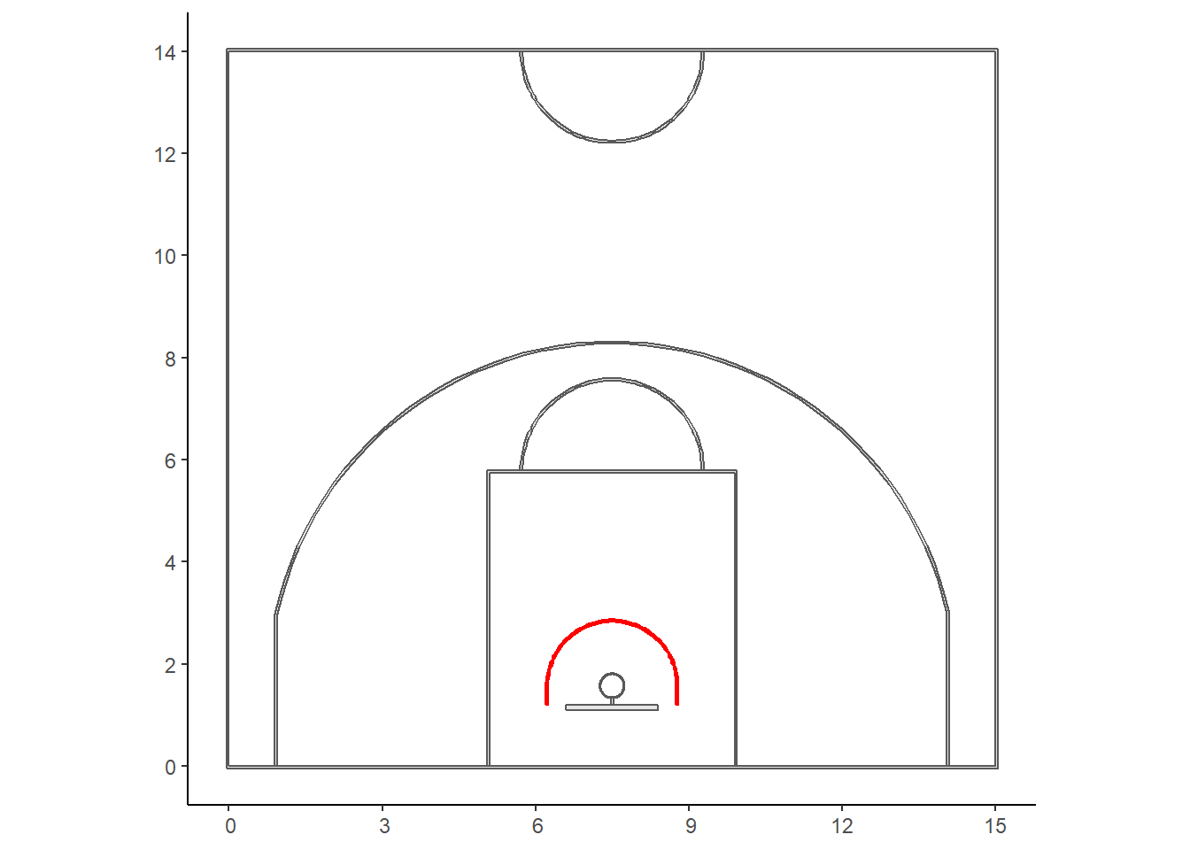

5.2 Creating an sf object

Lastly, we can create an sf object using st_sf() with all the different sfg objects we created.

# Create sf object with 9 features and 1 field
court_sf <- st_sf(
  description = c("half_court", "key", "hoop", "backboard",
                  "neck", "key_circle", "three_point_line",
                  "half_circle", "restricted_area"), 
  geom = c(st_geometry(half_court), st_geometry(key), st_geometry(hoop),
           st_geometry(backboard), st_geometry(neck), st_geometry(key_circle), 
           st_geometry(three_point_line), st_geometry(half_circle),
           st_geometry(restricted_area))
)

# Print sf object
court_sf

## Simple feature collection with 9 features and 1 field
## Geometry type: POLYGON
## Dimension:     XY
## Bounding box:  xmin: -0.05 ymin: -0.05 xmax: 15.05 ymax: 14.05
## CRS:           NA
##        description                           geom
## 1       half_court POLYGON ((-0.05 -0.05, -0.0...
## 2              key POLYGON ((5.05 0, 5.05 5.8,...
## 3             hoop POLYGON ((7.745 1.575, 7.74...
## 4        backboard POLYGON ((6.6 1.1, 6.6 1.2,...
## 5             neck POLYGON ((7.475 1.2, 7.475 ...
## 6       key_circle POLYGON ((5.702467 5.894205...
## 7 three_point_line POLYGON ((0.95 0, 0.95 2.99...
## 8      half_circle POLYGON ((9.297533 13.9058,...
## 9  restricted_area POLYGON ((6.2 1.2, 6.2 1.57...

We see that the bounding box of the court_sf object matches the court dimensions and the line thickness. Our spatial object has 9 features (polygons) and 1 field (description).

5.3 Plotting an`sf object

We can now easily plot and customize our basketball court.

# Plot a funky court with different colors for each feature
ggplot() +
  geom_sf(data = court_sf,  
          aes(fill = factor(description), color = factor(description))) +
  theme_classic() +
  scale_fill_discrete(name = "Feature") +
  scale_colour_discrete(guide = FALSE)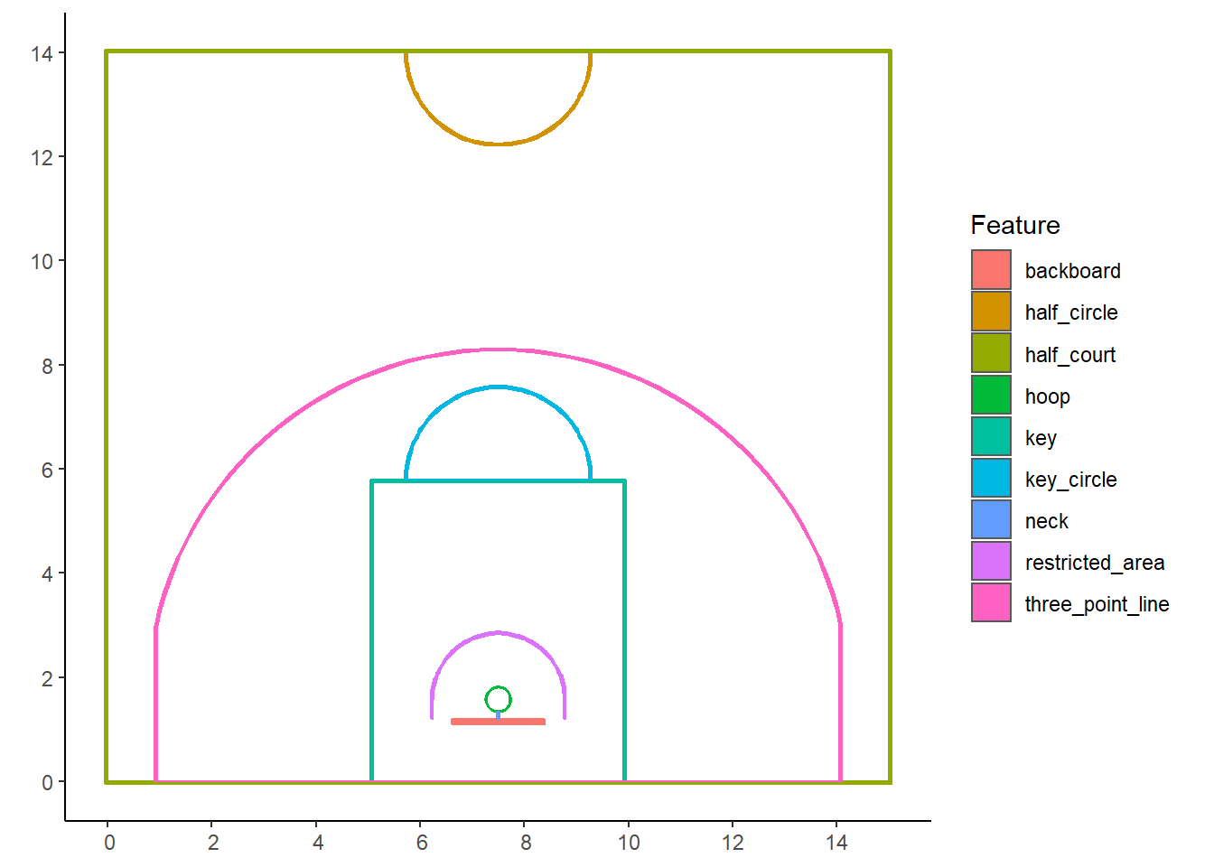

Figure 5.8: Funky basketball court

We can also define a function that will allow us to plot a court without needing to generate the court points each time.

plot_court = function(court_theme = court_themes$light) {
  ggplot() +
    geom_sf(data = court_sf,
            fill = court_theme$lines, col = court_theme$lines) +
    theme_void() +
    theme(
      text = element_text(color = court_theme$text),
      plot.background = element_rect(
        fill = court_theme$court, color = court_theme$court),
      panel.background = element_rect(
        fill = court_theme$court, color = court_theme$court),
      panel.grid = element_blank(),
      panel.border = element_blank(),
      axis.text = element_blank(),
      axis.title = element_blank(),
      axis.ticks = element_blank(),
      legend.background = element_rect(
        fill = court_theme$court, color = court_theme$court),
      legend.margin = margin(-1, 0, 0, 0, unit = "lines"),
      legend.position = "bottom",
      legend.key = element_blank(),
      legend.text = element_text(size = rel(1.0))
    )
}

# Light Theme (Default)
plot_court()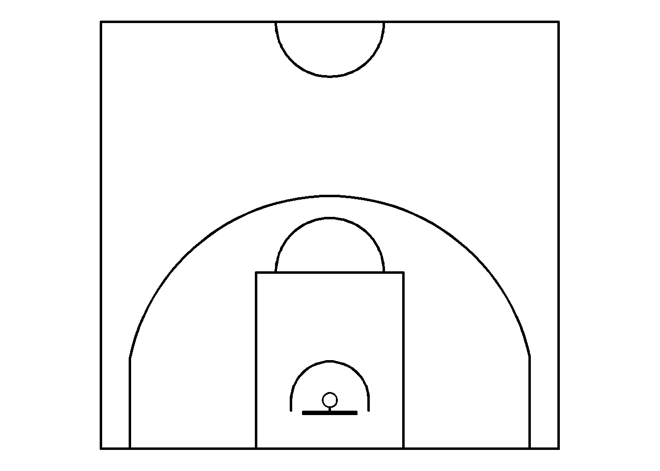

Figure 5.9: Light theme

# Dark Theme
plot_court(court_theme = court_themes$dark)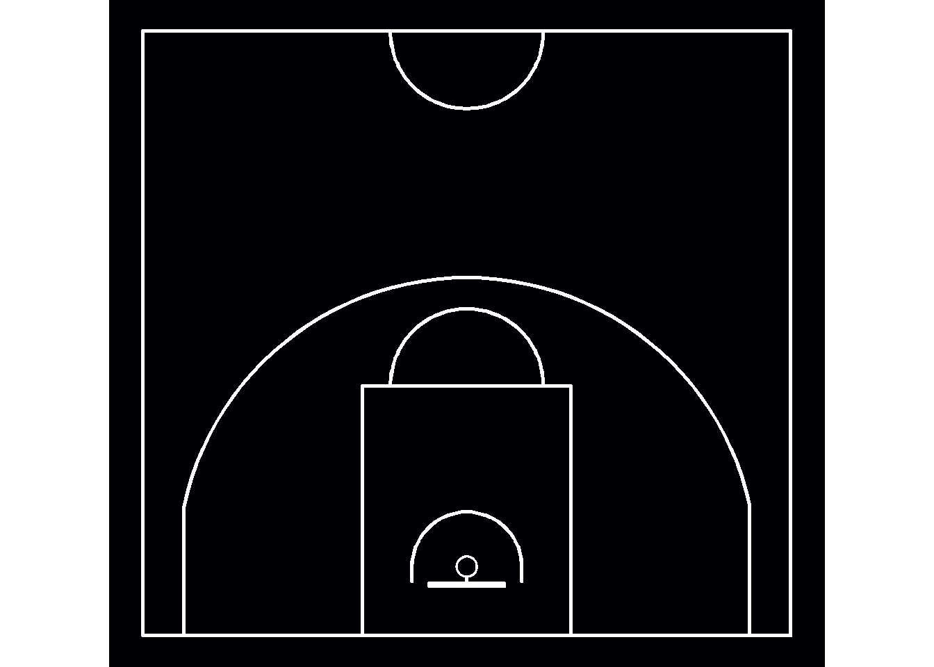

Figure 5.10: Dark theme

We are now able to plot an accurate basketball court using ggplot2 and the sf package using one line of code; plot_court().

We will see in the next chapter how we can convert our shot data into a spatial object to analyze and plot the shots using the sf package.

Note that all the R code used in this book is accessible on GitHub.